Joining Data in SQL Using PostgreSQL¶

Course: DataCamp: Joining Data in SQL Notebook Author: Jae Choi

Course Description

In this course you'll learn all about the power of Joining tables while exploring interesting features of countries and their cities throughout the world. You will master Inner and outer Joins, as well as self-Joins, semi-Joins, anti-Joins and cross Joins - fundamental tools in any PostgreSQL wizard's toolbox. You'll fear set theory no more, after learning all about unions, intersections, and except clauses through easy-to-understand diagrams and examples. Lastly, you'll be introduced to the challenging topic of subqueries. You will see a visual perspective to grasp the ideas throughout the course Using the mediums of Venn diagrams and other linking illustrations.

Datasets

Countries Leaders Diagrams

Imports

# 1. magic to print version
# 2. magic so that the notebook will reload external python modules
# https://gist.github.com/minrk/3301035
%load_ext watermark
%load_ext autoreload
%autoreload
import psycopg2
from sqlalchemy import create_engine
from sqlalchemy import MetaData
from sqlalchemy import Table
from sqlalchemy import Column
from sqlalchemy import Integer, String
from sqlalchemy import inspect
import pandas as pd
from pprint import pprint as pp
%watermark -a 'Jae H. Choi' -d -t -v -p psycopg2,sqlalchemy,pandas

Jae H. Choi 2020-08-30 19:19:16

CPython 3.8.3
IPython 7.16.1

psycopg2 2.8.5
sqlalchemy 1.3.18
pandas 1.0.5

PandAs Configuration Options

pd.set_option('max_columns', 200)
pd.set_option('max_rows', 300)
pd.set_option('display.expand_frame_repr', True)

PostgreSQL Connection

In order to run this Notebook, install, setup and configure a PostgreSQL databAse with the previously mentioned datAsets. Edit engine to use your databAse username and pAssword.

t_host = "localhost" #"databAse address"
t_port = "5432" #default postgres port
t_dbname = "datacamp" #"databAse name"
t_user = "postgres" #"databAse user name"
t_pw = "1234" #"databAse user pAssword"
db_conn = psycopg2.connect(host=t_host, database=t_dbname, user=t_user, password=t_pw)
# Scheme: "postgres+psycopg2://<USERNAME>:<PASSWORD>@<IP_ADDRESS>:<PORT>/<DATABASE_NAME>"
engine = create_engine('postgresql+psycopg2://postgres:1234@localhost/datacamp')

# metadate
meta = MetaData(schema="countries")
# connection
conn = engine.connect()

Example(s) without pd.DataFrames - use fetchall

result = conn.execute("Select datname From pg_database")
rows = result.fetchall()
[x for x in rows]

[('postgres',),
 ('template1',),
 ('template0',),
 ('northwind',),
 ('dds_assignment1',),
 ('ddsassignment2',),
 ('ddsassignment3',),
 ('datacamp',)]

# schema.table_name
cities = conn.execute("Select * \
            From countries.countries \
            Inner Join countries.cities \
            On countries.cities.country_code = countries.code")

cities_res = cities.fetchall()
cities_list = [x for i, x in enumerate(cities_res) if i < 10]

cities_list

[('CIV', "Cote d'Ivoire", 'Africa', 'Western Africa', 322463.0, 1960, 'Cote d\x92Ivoire', 'Republic', 'Yamoussoukro', -4.0305, 5.332, 'Abidjan', 'CIV', 4765000.0, None, 4765000.0),
 ('ARE', 'United Arab Emirates', 'Asia', 'Middle East', 83600.0, 1971, 'Al-Imarat al-´Arabiya al-Muttahida', 'Emirate Federation', 'Abu Dhabi', 54.3705, 24.4764, 'Abu Dhabi', 'ARE', 1145000.0, None, 1145000.0),
 ('NGA', 'Nigeria', 'Africa', 'Western Africa', 923768.0, 1960, 'Nigeria', 'Federal Republic', 'Abuja', 7.48906, 9.05804, 'Abuja', 'NGA', 1235880.0, 6000000.0, 1235880.0),
 ('GHA', 'Ghana', 'Africa', 'Western Africa', 238533.0, 1957, 'Ghana', 'Republic', 'Accra', -0.20795, 5.57045, 'Accra', 'GHA', 2070463.0, 4010054.0, 2070463.0),
 ('ETH', 'Ethiopia', 'Africa', 'Eastern Africa', 1104300.0, -1000, 'YeItyop´iya', 'Republic', 'Addis Ababa', 38.7468, 9.02274, 'Addis Ababa', 'ETH', 3103673.0, 4567857.0, 3103673.0),
 ('IND', 'India', 'Asia', 'Southern and Central Asia', 3287260.0, 1947, 'Bharat/India', 'Federal Republic', 'New Delhi', 77.225, 28.6353, 'Ahmedabad', 'IND', 5570585.0, None, 5570585.0),
 ('EGY', 'Egypt', 'Africa', 'Northern Africa', 1001450.0, 1922, 'Misr', 'Republic', 'Cairo', 31.2461, 30.0982, 'Alexandria', 'EGY', 4616625.0, None, 4616625.0),
 ('DZA', 'Algeria', 'Africa', 'Northern Africa', 2381740.0, 1962, 'Al-Jaza\x92ir/Algerie', 'Republic', 'Algiers', 3.05097, 36.7397, 'Algiers', 'DZA', 3415811.0, 5000000.0, 3415811.0),
 ('KAZ', 'Kazakhstan', 'Asia', 'Southern and Central Asia', 2724900.0, 1991, 'Qazaqstan', 'Republic', 'Astana', 71.4382, 51.1879, 'Almaty', 'KAZ', 1703481.0, None, 1703481.0),
 ('TUR', 'Turkey', 'Asia', 'Middle East', 774815.0, 1923, 'Turkiye', 'Republic', 'Ankara', 32.3606, 39.7153, 'Ankara', 'TUR', 5271000.0, 4585000.0, 5271000.0)]

1. Introduction to Joins¶

In this chapter, you'll be introduced to the concept of Joining tables, and explore the different ways you can enrich your queries Using Inner Joins and self-Joins. You'll also see how to use the cAse statement to split up a field into different categories.

1.1. Introduction to Inner Join¶

cities = conn.execute("Select * From countries.cities")
cities_df = pd.read_sql("Select * From countries.cities", conn)
cities_df.head()

sql_stmt = "Select * \
            From countries.cities \
            Inner Join countries.countries \
            ON countries.cities.country_code = countries.countries.code"
pd.read_sql(sql_stmt, conn).head()

sql_stmt = "Select countries.cities.name As city, \
                   countries.countries.name As country, \
                   countries.countries.region \
            From countries.cities \
            Inner Join countries.countries ON \
            countries.cities.country_code = countries.countries.code"
pd.read_sql(sql_stmt, conn).head()

1.2. Inner Join via Using¶

Select left_table As L_id
left_table.val As L_val
right_table.val As R_val
From left_table
Inner Join right_table
ON left_table.id=right_table.id;

- When the key field you'd like to Join on is the same name in both tables, you can use a Using clause instead of the ON clause.

Select left_table.id As L_id
left_table.val As L_val
right_table.val As R_val
From left_table
Inner Join right_table
Using (id);

1.2.1. Countries with prime ministers and presidents¶

Select p1.country,p1.continent,prime_minister,president
From leaders.presidents As p1
Inner Join leaders.prime_ministers As p2
Using (country);

sql_stmt = "Select p1.country, p1.continent, prime_minister, president \
            From leaders.presidents As p1 \
            Inner Join leaders.prime_ministers As p2 \
            Using (country)"

pd.read_sql(sql_stmt, conn).head()

1.2.2. Exercises¶

1.2.2.1. Review Inner Join Using on¶

Why does the following code result in an error?

Select c.name As country,
l.name As language
From countries As c
Inner Join languages As l;

Inner Join requires a specification of the key field (or fields) in each table.

1.2.2.2. Inner Join with Using¶

When Joining tables with a common field name, e.g.

Select *
From countries
Inner Join economies
ON countries.code=economies.code;

You can use Using As a shortcut:

Select *
From countries
Inner Join economies
Using (code);

You'll now explore how this can be done with the countries and languages tables.

Instructions

Inner Join countries on the left and languages on the right with Using(code).
Select the fields corresponding to:
- country name As country,
- continent name,
- language name As language, and
- whether or not the language is official.
Remember to aliAs your tables Using the first letter of their names.

-- Select fields and field's name as 'country'
Select c.name As country,
c.continent,
l.name As language,
l.official
-- From countries (alias As c)
From countries As c
-- Join to languages (As l)
Inner Join languages As l
-- Match Using code
Using (code);

sql_stmt = "Select c.name As country, \
                    c.continent, \
                    l.name As language, \
                    l.official \
From countries.countries As c \
Inner Join countries.languages As l \
Using (code)"

pd.read_sql(sql_stmt, conn).head()

1.3. Self Joins, just in CASE¶

1.3.1. self-Join on prime_ministers¶

sql_stmt = "Select * \
From leaders.prime_ministers"

pm_df = pd.read_sql(sql_stmt, conn)
pm_df.head()

Inner Joins where a table is Joined with itself
- self Join

Explore how to slice a numerical field into categories using the CASE command
Self-Joins are used to compare values in a field to other values of the same field From within the same table
Recall the prime ministers table:
- What if you wanted to create a new table showing countries that are in the same continenet matched As pairs?

Select p1.country As country1,
p2.country, As country2,
p1.continent
From leaders.prime_ministers As p1
Inner Join prime_ministers As p2
On p1.continent=p2.continent;

sql_stmt = "Select p1.country As country1, \
                   p2.country As country2, \
                   p1.continent \
From leaders.prime_ministers As p1 \
Inner Join leaders.prime_ministers As p2 \
ON p1.continent = p2.continent"

pm_df_1 = pd.read_sql(sql_stmt, conn)
pm_df_1.head()

The country column is Selected twice As well As continent.
The prime ministers table is on both the left and the right.
The vital step is setting the key columns by which we match the table to itself.
- For each country, there will be a match if the country in the right table p2 (prime_ministers) is in the same continent.
This is a pairing of each country with every other country in its same continent
- Conditions where country1 = country2 should not be included in the table

1.3.2. Finishing off the self-Join on prime_ministers¶

Select p1.country As country1,
p2.country As country2,
p1.continent
From leaders.prime_ministers As p1
Inner Join prime_ministers As p2
On p1.continent=p2.continent
And p1.country!=p2.country;

sql_stmt = "Select p1.country As country1, \
                   p2.country As country2, \
                   p1.continent \
From leaders.prime_ministers As p1 \
Inner Join leaders.prime_ministers As p2 \
ON p1.continent = p2.continent AND p1.country != p2.country"

pm_df_2 = pd.read_sql(sql_stmt, conn)
pm_df_2.head()

pm_df_1.equals(pm_df_2)

False

And clause can check that multiple conditions are met.
Now a match will not be made between prime_minister and itself if the countries match

1.3.3. CASE WHEN and THEN¶

The states table contains numeric data about different countries in the six inhabited world continents
Group the year of independence into categories of:
- before 1900
- between 1900 and 1930
- and after 1930

Case is a way to do multiple if-then-else statements

Select name,continent,indep_year,
Case When indep_year < 1900 Then 'before 1900'
When indep_year <= 1930 Then 'between 1900 and 1930'
Else 'after 1930' End
As indep_year_group
From states
Order By indep_year_group;

sql_stmt = "Select name, continent, indep_year, \
    Case When indep_year < 1900 Then 'before 1900' \
        When indep_year <= 1930 Then 'between 1900 and 1930' \
        Else 'after 1930' End \
        As indep_year_group \
    From leaders.states \
    Order By indep_year_group"

pd.read_sql(sql_stmt, conn)

1.3.4. Exercises¶

1.3.4.1. Self-Join¶

In this exercise, you'll use the populations table to perform a self-Join to calculate the percentage increAse in population From 2010 to 2015 for each country code! Since you'll be Joining the populations table to itself, you can aliAs populations As p1 and also populations As p2. This is good practice whenever you are aliAsing and your tables have the same first letter. Note that you are required to aliAs the tables with self-Joins.

Instructions 1)

Join populations with itself ON country_code.
Select the country_code From p1 and the size field From both p1 and p2. SQL won't allow same-named fields, so aliAs p1.size As size2010 and p2.size As size2015.

-- Select fields with aliases
Select p1.size As size2010,
p1.country_code,
p2.size As size2015,
-- From populations (alias As p1)
From countries.populations As p1
-- Join to itself (alias As p2)
Inner Join countries.populations As p2
-- Match on country code
On p1.country_code=p2.country_code;

sql_stmt = "Select p1.size As size2010, \
                    p1.country_code, \
                    p2.size As size2015 \
From countries.populations As p1 \
Inner Join countries.populations As p2 \
On p1.country_code = p2.country_code"

pd.read_sql(sql_stmt, conn).head()

Instructions 2) Notice From the result that for each country_code you have four entries laying out all combinations of 2010 and 2015.

Extend the On in your query to include only those records where the p1.year (2010) matches with p2.year - 5 (2015 - 5 = 2010). This will omit the three entries per country_code that you aren't interested in.

-- Select fields with aliases
Select p1.country_code,
p1.size As size2010,
p2.size As size2015
-- From populations (alias As p1)
From countries.populations As p1
-- Join to itself (alias As p2)
Inner Join countries.populations As p2
-- Match on country code
On p1.country_code=p2.country_code
-- and year (with calculation)
And p1.year=(p2.year-5);

sql_stmt = "Select p1.size As size2010, \
                    p1.country_code, \
                    p2.size As size2015 \
From countries.populations As p1 \
Inner Join countries.populations As p2 \
ON p1.country_code = p2.country_code \
    AND p1.year = (p2.year - 5)"

pd.read_sql(sql_stmt, conn).head()

Instructions 3)

As you just saw, you can also use SQL to calculate values like p2.year - 5 for you. With two fields like size2010 and size2015, you may want to determine the percentage increAse From one field to the next: With two numeric fields A and B, the percentage growth From A to B can be calculated As $$\frac{(B−A)}{A}∗100.0$$.

Add a new field to Select, aliased As growth_perc, that calculates the percentage population growth From 2010 to 2015 for each country, Using p2.size and p1.size.

Select p1.country_code,
p1.size As size2010,
p2.size As size2015,
-- calculate growth_perc
(p2.size-p1.size)/p1.size*100.0 As growth_perc
-- From populations (alias As p1)
From countries.populations As p1
-- Join to itself (alias As p2)
Inner Join countries.populations As p2
-- Match on country code
On p1.country_code=p2.country_code
-- and year (with calculation)
And p1.year=p2.year-5;

sql_stmt = "Select p1.size As size2010, \
                    p1.country_code, \
                    p2.size As size2015, \
            (p2.size - p1.size)/p1.size * 100.0 As growth_perc \
From countries.populations As p1 \
Inner Join countries.populations As p2 \
ON p1.country_code = p2.country_code \
AND p1.year = (p2.year - 5)"

pd.read_sql(sql_stmt, conn).head()

1.3.4.2. Case-When-and-Then">CAse when and then¶

Often it's useful to look at a numerical field not As raw data, but instead As being in different categories or groups. You can use Case with When, Then, Elese, and End to define a new grouping field.

Instructions

Using the countries table, create a new field As geosize_group that groups the countries into three groups:

If surface_area is greater than 2 million, geosize_group is 'large'. If surface_area is greater than 350 thousand but not larger than 2 million, geosize_group is 'medium'. Otherwise, geosize_group is 'small'.

Select name, continent, code, surface_area,
-- First case
Case When surface_area > 2000000 Then 'large'
-- Second case
When surface_area > 350000 Then 'medium'
-- Else clause + End
Else 'small' END
-- Alias name
As geosize_group
-- From table
From countries.countries;

sql_stmt = "Select name, continent, code, surface_area, \
                Case When surface_area > 2000000 Then 'large' \
                    When surface_area > 350000 Then 'medium' \
                    Else 'small' End \
                    As geosize_group \
From countries.countries;"

pd.read_sql(sql_stmt, conn).head()

1.3.4.3. Inner challenge¶

The table you created with the added geosize_group field hAs been loaded for you here with the name countries_plus. Observe the use of (and the placement of) the Into command to create this countries_plus table:

Select name,continent,code,surface_area,
Case When surface_area > 2000000 Then 'large'
When surface_area > 350000 Then 'medium'
Else 'small' End
As geosize_group Into countries_plus
From countries.countries;

You will now explore the relationship between the size of a country in terms of surface area and in terms of population Using grouping fields created with Case. By the end of this exercise, you'll be writing two queries back-to-back in a single script. You got this!

Instructions 1) Using the populations table focused only for the year 2015, create a new field As popsize_group to organize population size into

'large' (> 50 million)
'medium' (> 1 million)
'small' (<= 1 million)

Select only the country code, population size, and this new popsize_group As fields.

Select country_code,size,
-- First case
Case When size>50000000 Then 'large'
-- Second case
When size>1000000 Then 'medium'
-- Else clause + End
Else 'small' End
-- Alias name
As popsize_group
-- From table
From countries.populations
-- Focus on 2015
Where year=2015;

sql_stmt = "Select country_code, size, \
                Case When size > 50000000 Then 'large' \
                    When size > 1000000 Then 'medium' \
                    Else 'small' End \
                    As popsize_group \
From countries.populations \
Where year = 2015;"

pd.read_sql(sql_stmt, conn).head()

Execute the first part on the PostgreSQL schema to create pop_plus

#CREATE TABLE new_table
#  AS (SELECT *
#      FROM old_table WHERE 1=2)

sql_stmt = "Create Table countries.pop_plus \
                As (Select country_code, size, \
                        Case When size > 50000000 Then 'large' \
                        When size > 1000000 Then 'medium' \
                        Else 'small' End \
                        As popsize_group \
                    From countries.populations \
                    Where year = 2015);"
engine.execute(sql_stmt)

<sqlalchemy.engine.result.ResultProxy at 0x104fe1d30>

Instructions 2)

Use Into to save the result of the previous query As pop_plus. You can see an example of this in the countries_plus code in the Assignment text. Make sure to include a ; at the end of your Where clause!
Then, include another query below your first query to display all the records in pop_plus Using Select * From pop_plus; so that you generate results and this will display pop_plus in query result.

Select country_code,size,
Case When size>50000000 Then 'large'
When size>1000000 Then 'medium'
Else 'small' End
As popsize_group
-- Into table
Into countries.pop_plus
From populations
Where year=2015;

sql_stmt="Select country_code,size,\
                Case When size>50000000 Then 'large'\
                    When size>1000000 Then 'medium'\
                    Else 'small' End\
                    As popsize_group\
                    Into countries.test1\
            From populations\
            Where year=2015;"
engine.execute(sql_stmt)

<sqlalchemy.engine.result.ResultProxy at 0x115fdabb0>

sql_stmt = "\
SELECT * FROM countries.pop_plus; \
"

pd.read_sql(sql_stmt, conn).head()

Instructions 3)

Keep the first query intact that creates pop_plus using Into.
Write a query to Join countries_plus As c on the left with pop_plus As p on the right matching on the country code fields.
Sort the data based on geosize_group, in Ascending order so that large appears on top.
Select the name, continent, geosize_group, and popsize_group fields.

sql_stmt = "\
Select c.name, c.continent, c.geosize_group, p.popsize_group \
From countries.countries_plus As c \
Inner Join countries.pop_plus As p \
ON c.code = p.country_code \
ORDER BY geosize_group AsC \
"

q_df = pd.read_sql(sql_stmt, conn)
q_df.head()

q_df.tail()

2. Outer Joins and Cross Joins¶

In this chapter, you'll come to grips with different kinds of outer Joins. You'll learn how to gain further insights into your data through left Joins, right Joins, and full Joins. In addition to outer Joins, you'll also work with cross Joins.

2.1. LEFT and RIGHT Joins¶

You can remember outer Joins As reaching out to another table while keeping all of the records of the original table.
Inner Joins keep only the records in both tables.
This chapter will explore three types of OUTER Joins:
1. How a LEFT Join differs From an Inner Join:

Inner Join

Select p1.country
prime_minister,
president
From prime_ministers As p1
Inner Join presidents As p2
On p1.country=p2.country;

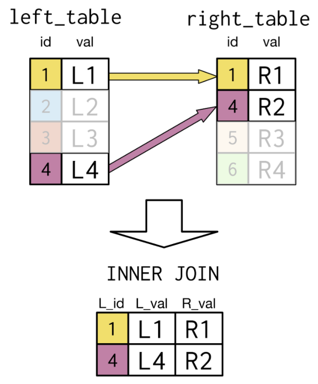
The only records included in the resulting table of the Inner Join query were those in which the id field had matching values.

LEFT Join

Select p1.country
prime_minister,
president
From prime_ministers As p1
Left Join presidents As p2
On p1.country=p2.country;

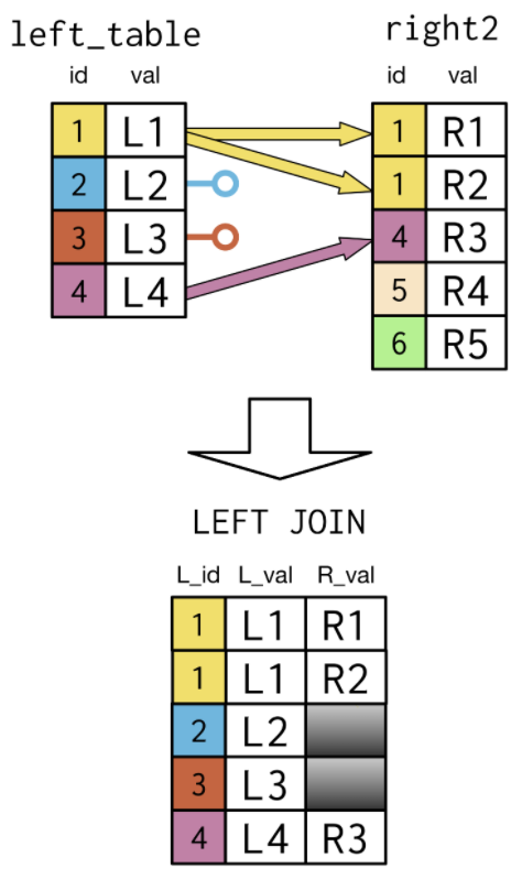
In contrast, a LEFT Join notes those record in the left table that do not have a match on the key field in the right table.
This is denoted in the diagram by the open circles remaining close to the left table for id values of 2 and 3.
Whereas the Inner Join kept just the records corresponding to id values 1 and 44, a LEFT Join keeps all of the original records in the left table, but then marks the values as missing in the right table for those that don't have a match.
The syntax of the LEFT Join is similar to that of the Inner Join.

LEFT Join multiple matches

It isn't always the case that each key value in the left table corresponds to exactly one record in the key column of the right table.
Duplicate rows are shown in the LEFT Join for id 1 since it hAs two matches corresponding to the values of R1 and R2 in the right2 table.

RIGHT Join

Select right_table.id As R_id
left_table.val As L_val,
right_table.val As R_val,
From left_table
Right Join right_table
On left_table.id=right_table.id;

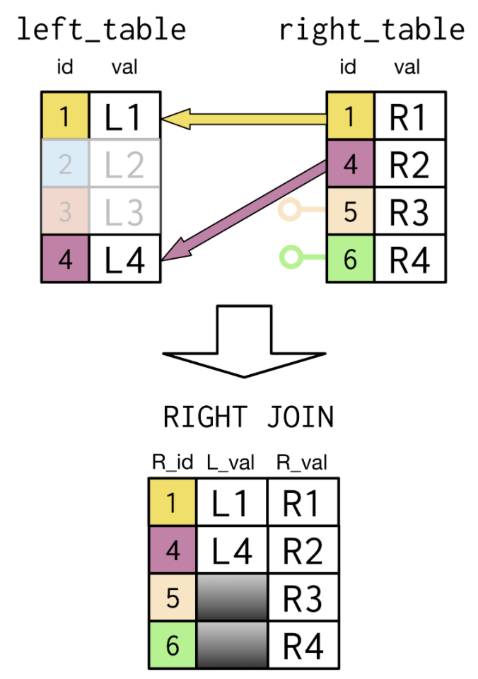
Instead of matching entries in the id column on the left table to the id column on the right table, a RIGHT Join does the reverse.
- The resulting table From a RIGHT Join shows the missing entries in the L_val field.
In the SQL statement the right table appears after RIGHT Join and the left table appears after From.

2.1.1. Inner Join¶

sql_stmt = "Select p1.country, \
                prime_minister, \
                president \
From leaders.prime_ministers As p1 \
Inner Join leaders.presidents As p2 \
ON p1.country = p2.country"

pd.read_sql(sql_stmt, conn)

2.1.2. LEFT Join¶

The first four records are the same as those From Inner Join
The following records correspond to the countries that do not have a president and thus their president values are missing.

sql_stmt = "Select p1.country, prime_minister, president \
From leaders.prime_ministers As p1 \
LEFT Join leaders.presidents As p2 \
ON p1.country = p2.country"

pd.read_sql(sql_stmt, conn)

2.1.3. Exercises¶

2.1.3.1. LEFT Join¶

Now you'll explore the differences between performing an Inner Join and a left Join Using the cities and countries tables. You'll begin by performing an Inner Join with the cities table on the left and the countries table on the right. Remember to aliAs the name of the city field As city and the name of the country field As country. You will then change the query to a left Join. Take note of how many records are in each query here!

Instructions 1)

Fill in the code bAsed on the instructions in the code comments to complete the Inner Join. Note how many records are in the result of the Join in the query result tab.

-- Select the city name (with alias), the country code, the country name (with alias), the region, and the city proper population
Select c1.name As city,
code,
c2.name, As country,
region,
city_proper_pop,
-- From left table (with alias)
From cities As c1
-- Join to right table (with alias)
Inner Join countries As c2
-- Match on country code
On c1.country_code=c2.code
Order By code Desc;

sql_stmt = "Select c1.name As city, \
                    code, \
                    c2.name As country, \
                    region, city_proper_pop \
From countries.cities As c1 \
Inner Join countries.countries As c2 \
ON c1.country_code = c2.code \
ORDER BY code DESC;"

pd.read_sql(sql_stmt, conn).head()

Instructions 2)

Change the code to perform a LEFT Join instead of an Inner Join. After executing this query, note how many records the query result contains.

Select c1.name As city,
code,
c2.name, As country,
region,
city_proper_pop,
From cities As c1
-- Join to right table (with alias)
Left Join countries As c2
-- Match on country code
On c1.country_code=c2.code
Order By code Desc;

sql_stmt = "Select c1.name As city, \
                    code, \
                    c2.name As country,\
                    region, city_proper_pop \
From countries.cities As c1 \
LEFT Join countries.countries As c2 \
ON c1.country_code = c2.code \
ORDER BY code DESC;"

pd.read_sql(sql_stmt, conn).head()

2.1.3.2. JEFT Join (2)¶

Next, you'll try out another example comparing an Inner Join to its corresponding left Join. Before you begin though, take note of how many records are in both the countries and languages tables below.

You will begin with an Inner Join on the countries table on the left with the languages table on the right. Then you'll change the code to a left Join in the next bullet.

Note the use of multi-line comments here Using /* and */.

Instructions 1)

Perform an Inner Join. AliAs the name of the country field As country and the name of the language field As language.
Sort bAsed on desc

sql_stmt = "Select c.name As country, \
                    local_name, \
                    l.name As language, \
                    percent \
From countries.countries As c \
Inner Join countries.languages As l \
On c.code = l.code \
Order By country Desc; "

res1 = pd.read_sql(sql_stmt, conn)
print(f'Number of Records: {len(res1)}')
res1.head()

Number of Records: 914

Instructions 2)

Perform a left Join instead of an Inner Join. Observe the result, and also note the change in the number of records in the result.
Carefully review which records appear in the left Join result, but not in the Inner Join result.

sql_stmt = "Select c.name As country, \
                    local_name, \
                    l.name As language, \
                    percent \
From countries.countries As c \
LEFT Join countries.languages As l \
On c.code = l.code \
Order By country Desc; \
"

res2 = pd.read_sql(sql_stmt, conn)
print(f'Number of Records: {len(res2)}')
res2.head()

Number of Records: 921

2.1.3.3. LEFT Join (3)¶

You'll now revisit the use of the AVG() function introduced in our Intro to SQL for Data Science course. You will use it in combination with left Join to determine the average gross domestic product (GDP) per capita by region in 2010.

Instructions 1)

Begin with a left Join with the countries table on the left and the economies table on the right.
Focus only on records with 2010 As the year.

sql_stmt = "Select name, \
                region, \
                gdp_percapita \
From countries.countries As c \
LEFT Join countries.economies As e \
On e.code = c.code \
Where year = 2010; \
"

res1 = pd.read_sql(sql_stmt, conn)
print(f'Number of Records: {len(res1)}')
res1.head()

Number of Records: 185

Instructions 2)

Modify your code to calculate the average GDP per capita As avg_gdp for each region in 2010.
Select the region and avg_gdp fields.

sql_stmt = "Select region, \
                    AVG(gdp_percapita) As avg_gdp \
From countries.countries As c \
LEFT Join countries.economies As e \
On e.code = c.code \
Where year = 2010 \
Group BY region \
Order BY avg_gdp Desc; \
"

res2 = pd.read_sql(sql_stmt, conn)
print(f'Number of Records: {len(res2)}')
res2.head()

Number of Records: 23

Instructions 3)

Arrange this data on average GDP per capita for each region in 2010 From highest to lowest average GDP per capita.

sql_stmt = "Select region, \
            AVG(gdp_percapita) As avg_gdp \
From countries.countries As c \
LEFT Join countries.economies As e \
On e.code = c.code \
Where year = 2010 \
Group BY region;"

res3 = pd.read_sql(sql_stmt, conn)
print(f'Number of Records: {len(res3)}')
res3.head()

Number of Records: 23

2.1.3.4. RIGHT Join¶

Right Joins aren't As common As left Joins. One reAson why is that you can always write a right Join As a left Join.

Instructions

The left Join code is commented out here. Your tAsk is to write a new query Using rights Joins that produces the same result As what the query Using left Joins produces. Keep this left Joins code commented As you write your own query just below it Using right Joins to solve the problem.
Note the order of the Joins matters in your conversion to Using right Joins!
convert this code to use RIGHT Joins instead of LEFT Joins

Select cities.name As city,
urbanarea_pop,
countries.name, As country,
languages.name As language,
percent
From cities
Left Join countries
On cities.country_code=countries.code
Left Join languages
On countries.code=languages.code
Order By city, language;

sql_stmt = "Select cities.name As city,\
                    urbanarea_pop, \
                    countries.name As country, \
                    indep_year, \
                    languages.name As language, \
                    percent \
From countries.languages \
Left Join countries.countries \
On languages.code = countries.code \
Left Join countries.cities \
On cities.country_code = countries.code \
Order BY city, language; \
"

pd.read_sql(sql_stmt, conn).head()

2.2. FULL Joins¶

The last of the three types of OUTER Joins is the FULL Join
Explore the difference between FULL Join and other Joins
- The instruction will focus on comparing them to Inner Joins and LEFT Joins and then to LEFT Joins and RIGHT Joins.
Let's review how the diagram changes between and Inner Join and a LEFT Join for our bAsic example Using the left and right tables.
Then we'll delve into the FULL Join diagram and is SQL code.

Recall that an Inner Join keeps only the records that have matching key field values in both tables.

A LEFT Join keeps all of the records in the left table while bringing in missing values for those key field values that don't appear in the right table.

Let's review the differences between a LEFT Join and a RIGHT Join.
The id values of 2 and 3 in the left table do not match with the id values in the right table, so missing values are brought in for them in the LEFT Join.
Likewise for the RIGHT Join, missing values are brought in for id values of 5 and 6.

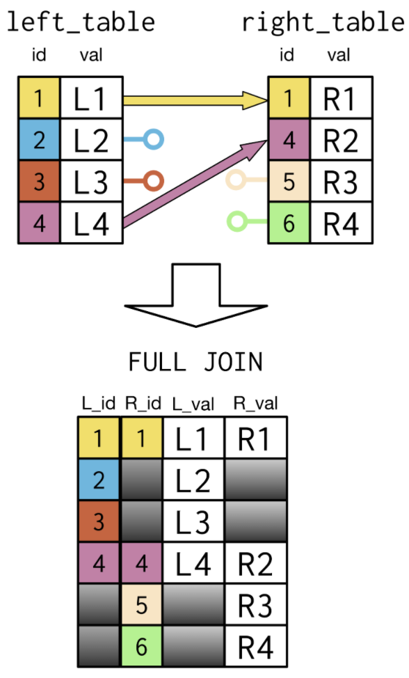
A FULL Join combines a LEFT Join and RIGHT Join As you can see in the diagram.

Select left_table.id As L_id,
right_table.id As R_id,
left_table.val, As L_val,
right_table.val As R_val
From left_table
Full Join right_table
Using (id);

It will bring in all record From both the left and the right table and keep track of the missing values accordingly.
Note the missing values here and all six of the values of id are included in the table.
You can also see From the SQL code, to produce this FULL Join result, the general format aligns closely with the SQL syntax seen for an Inner Join and a LEFT Join.

2.2.1. FULL Join example using leaders database¶

Let's revisit the example of looking at countries with prime ministers and / or presidents.
Query breakdown:
- The Select statement includes the country field From both tables of interest and also the prime_minister and president fields.
- The left table is specified As prime_ministers with the aliAs of p1
- The order matters and if you switched the two tables, the output would be slightly different.
- The right table is specified As presidents with the aliAs of p2
- The Join is done bAsed on the key field of country in both tables

Select p1.country As pm_co,
p2.country As pres_co,
prime_minister,
president,
From prime_ministers As p1
Full Join presidents As p2
On p1.country=p2.country;

sql_stmt = "Select p1.country As pm_co,\
                    p2.country As pres_co, \
                    prime_minister, \
                    president \
From leaders.prime_ministers As p1 \
FULL Join leaders.presidents As p2 \
ON p1.country = p2.country;"

pd.read_sql(sql_stmt, conn)

2.2.2. Exercises¶

2.2.2.1. FULL Join¶

In this exercise, you'll examine how your results differ when Using a full Join versus Using a left Join versus Using an Inner Join with the countries and currencies tables.

You will focus on the North American region and also where the name of the country is missing. Dig in to see what we mean!

Begin with a full Join with countries on the left and currencies on the right. The fields of interest have been Selected for you throughout this exercise.

Then complete a similar left Join and conclude with an Inner Join.

Instructions 1)

Choose records in which region corresponds to North America or is NULL.

Select name As country,
code,
region,
basic_unit -- From to countries
From countries
-- Join to to currencies
Full Join currencies
Using (code)
-- Where region is North America or null
Where region='North America' Or region Is Null
; Order By region;

sql_stmt = "Select name As country, \
                    code, region, \
                    basic_unit \
From countries.countries \
FULL Join countries.currencies \
Using (code) \
Where region = 'North America' OR region Is Null \
Order BY region;"

pd.read_sql(sql_stmt, conn)

Instructions 2)

Repeat the same query As above but use a LEFT Join instead of a FULL Join. Note what hAs changed compared to the FULL Join result!
Select name As country,
code,
region,
basic_unit
-- From to countries
From countries
-- Join to to currencies
Left Join currencies
Using (code)
-- Where region is North America or null
Where region='North America' Or region Is Null
; Order By region;

sql_stmt = "Select name As country, \
                    code, region, basic_unit \
From countries.countries \
LEFT Join countries.currencies \
Using (code) \
Where region = 'North America' OR region Is Null \
ORder BY region;"

pd.read_sql(sql_stmt, conn)

Instruction 3)

Repeat the same query As above but use an Inner Join instead of a FULL Join. Note what hAs changed compared to the FULL Join and LEFT Join results!

Select name As country,
code,
region,
basic_unit
-- From countries
From countries
-- Join to to currencies
Inner Join currencies
Using (code)
-- Where region is North America or null
Where region='North America Or region Is Null
Order By region;

sql_stmt = "Select name As country, \
                    code, region, basic_unit \
From countries.countries \
Inner Join countries.currencies \
Using (code) \
Where region = 'North America' OR region IS null \
Order BY region; \
"

pd.read_sql(sql_stmt, conn)

Have you kept an eye out on the different numbers of records these queries returned? The FULL Join query returned 17 rows, the LEFT Join returned 4 rows, and the Inner Join only returned 3 rows. Do these results make sense to you?

2.2.2.3. FULL Join (2)¶

You'll now investigate a similar exercise to the last one, but this time focused on Using a table with more records on the left than the right. You'll work with the languages and countries tables. Begin with a full Join with languages on the left and countries on the right. Appropriate fields have been Selected for you again here. Instructions 1/3

Choose records in which countries.name starts with the capital letter 'V' or is NULL and arrange by countries.name in Ascending order to more clearly see the results.
Select name As country,
code,
languages.name As language
-- From languages
From languages
-- Join to to countries
Inner Join countries
Using (code)
-- Where region countries.name starts with V or is null
Where countries.name Like 'V%' Or countries.name Is Null
Order By countries.name;

sql_stmt = "Select countries.name, code, \
                    languages.name As language \
From countries.languages \
FULL Join countries.countries \
Using (code) \
Where countries.name LIKE 'V%%' OR countries.name IS null \
Order BY countries.name; \
"

pd.read_sql(sql_stmt, conn)

Instructions 2)

Repeat the same query As above but use a left Join instead of a full Join. Note what hAs changed compared to the full Join result!

Select countries.name As country,
code,
languages.name As language
-- From languages
From languages
-- Join to to countries
Left Join countries
Using (code)
-- Where countries.name starts with V or is null
Where countries.name Like 'V%' Or countries.name Is Null
Order By countries.name;

sql_stmt = "Select countries.name, code, \
                languages.name As language \
From countries.languages \
LEFT Join countries.countries \
Using (code) \
Where countries.name LIKE 'V%%' OR countries.name Is Null \
Order BY countries.name;"

pd.read_sql(sql_stmt, conn)

Instructions 3)

Repeat once more, but use an Inner Join instead of a left Join. Note what hAs changed compared to the full Join and left Join results.
Select countries.name As country,
code,
languages.name As language
-- From languages
From languages
-- Join to countries
Inner Join countries
Using (code)
-- Where countries.name starts with V or is null
Where countries.name Like 'V%' Or countries.name Is Null
Order By countries.name;

sql_stmt = "Select countries.name, code, \
                languages.name As language \
From countries.languages \
Inner Join countries.countries \
Using (code) \
Where countries.name Like 'V%%' OR countries.name IS null \
Order BY countries.name;"

pd.read_sql(sql_stmt, conn)

2.2.2.3. FULL Join (3)¶

You'll now explore Using two consecutive full Joins on the three tables you worked with in the previous two exercises.

Instructions

Complete a full Join with countries on the left and languages on the right.
Next, full Join this result with currencies on the right.
Use LIKE to choose the Melanesia and Micronesia regions (Hint: 'M%esia').
Select the fields corresponding to the country name As country, region, language name As language, and basic and fractional units of currency.

Select c1.name As country,
region,
l.name As language,
basic_unit,
frac_unit
-- From countries (alias as c1)
From countries As c1
-- Join to languages
Full Join languages As l
Using (code)
-- Join to currencies (alias as c1)
Full Join currencies As c2
Using (code)
-- Where region like Melanesia and Micronesia
Where region Like 'M%esia';

sql_stmt = "Select c1.name As country, region, \
                    l.name As language, \
                    basic_unit, frac_unit \
From countries.countries As c1 \
FULL Join countries.languages As l \
Using (code) \
FULL Join countries.currencies As c2 \
Using (code) \
Where region Like 'M%%esia';"

pd.read_sql(sql_stmt, conn)

2.2.2.4 Review OUTER Joins¶

A(n) ___ Join is a Join combining the results of a ___ Join and a ___ Join. Answer the question

~~left, full, right~~
~~right, full, left~~
~~Inner, left, right~~
None of the above are true</strong>

2.3. Cross-join¶

CROSS Joins create all possible combinations of two tables.

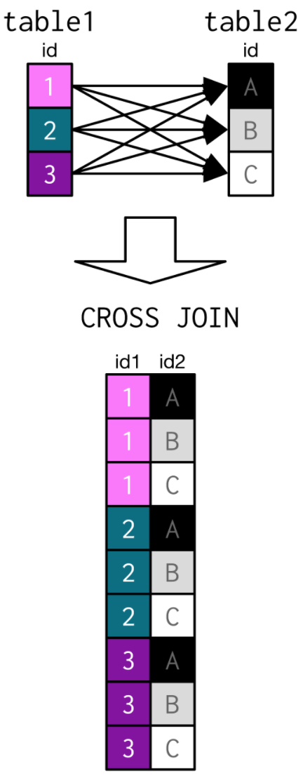
The resulting table is comprised of all 9 combinations if id From table1 and id From table2 (e.g. 1(A-C), 2(A-C), & 3(A-C))

2.3.1. CROSS Join example: Pairing prime ministers with presidents¶

Suppose all prime ministers in North America and Oceania in the prime_ministers table are scheduled for individual meetings with all presidents in the presidents table.
All the combinations can be created with a CROSS Join

Select prime_minister,
president,
From prime_ministers As p1
-- Join to languages
Cross Join presidents As p2
Where p1.continent In ('North America', 'Oceania');

sql_stmt = "Select prime_minister, \
                    president \
From leaders.prime_ministers As p1 \
CROSS Join leaders.presidents As p2 \
Where p1.continent IN ('North America', 'Oceania');"

pd.read_sql(sql_stmt, conn)

2.3.1.1. Exercises¶

A table of two cities

This exercise looks to explore languages potentially and most frequently spoken in the cities of Hyderabad, India and Hyderabad, Pakistan.

You will begin with a cross Join with cities As c on the left and languages As l on the right. Then you will modify the query Using an Inner Join in the next tab.

Instructions 1)

Create the cross Join As described above. (Recall that cross Joins do not use ON or Using.)
Make use of LIKE and Hyder% to choose Hyderabad in both countries.
Select only the city name As city and language name As language.

Select c.name As city,
l.name As language
From cities As c
Cross Join languages As l
Where c.name Like 'Hyder%';

sql_stmt = "Select c.name As city, \
                l.name As language \
From countries.cities As c \
CROSS Join countries.languages As l \
Where c.name Like 'Hyder%%';"

unique_lang = hyderabad_lang['language'].unique()
print(len(unique_lang))
hyderabad_lang = pd.read_sql(sql_stmt, conn)
hyderabad_lang

396

Instructions 2)

Use an Inner Join instead of a cross Join. Think about what the difference will be in the results for this Inner Join result and the one for the cross Join.

Select c.name As city,
l.name As language
From cities As c
Inner Join languages As l
On c.country_code=l.code
Where c.name Like 'Hyder%';

sql_stmt = "Select c.name As city, \
                l.name As language \
From countries.cities As c \
Inner Join countries.languages As l \
On c.country_code = l.code \
Where c.name LIKE 'Hyder%%';"

pd.read_sql(sql_stmt, conn)

Outer challenge

Now that you're fully equipped to use outer Joins, try a challenge problem to test your knowledge! In terms of life expectancy for 2010, determine the names of the lowest five countries and their regions.

Instructions

Select country name As country, region, and life expectancy As life_exp.
Make sure to use LEFT Join, Where, Order BY, and LIMIT.

Select c.name As country,
c.region,
p.life_expectancy As life_exp
From countries As c
Left Join populations As p
On c.code=l.country_code
Where p.year=2010
Order By life_exp Limit 5;

sql_stmt = "Select c.name As country, \
                    c.region, \
                    p.life_expectancy As life_exp \
From countries.countries As c \
LEFT Join countries.populations As p \
On c.code = p.country_code \
Where p.year = 2010 \
Order BY life_exp \
Limit 5;"

pd.read_sql(sql_stmt, conn)

3. Set theory clauses¶

In this chapter, you'll learn more about set theory Using Venn diagrams and you will be introduced to union, union all, intersect, and except clauses. You'll finish by investigating semi-Joins and anti-Joins, which provide a nice introduction to subqueries.

3.1. State of the UNION¶

Focus on the operations UNION and UNION ALL.
In addition to Joining diagrams, you'll see how Venn diagrams can be used to represent set operations.

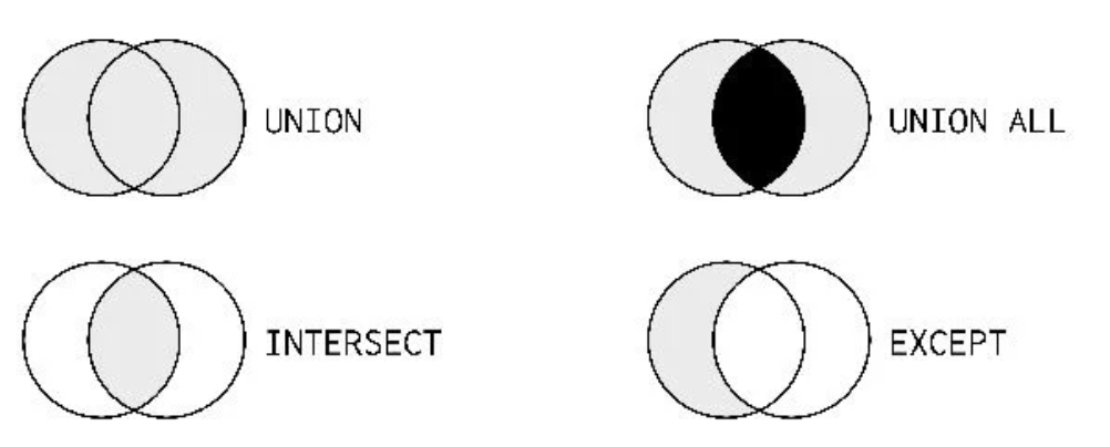
Think of each circle As representing a table of data
The shading represents what's included in the result of the set operation From each table.
UNION includes every record in both tables, but DOES NOT double count those that are in both tables.
UNION ALL includes every record in both tables and DOES replicate those that are in both tables, represented by the black center
The two diagrams on the bottom represent only the subsets of data being Selected.
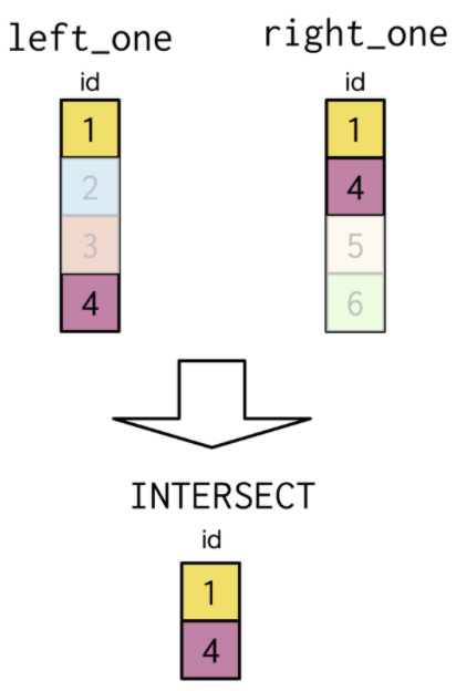
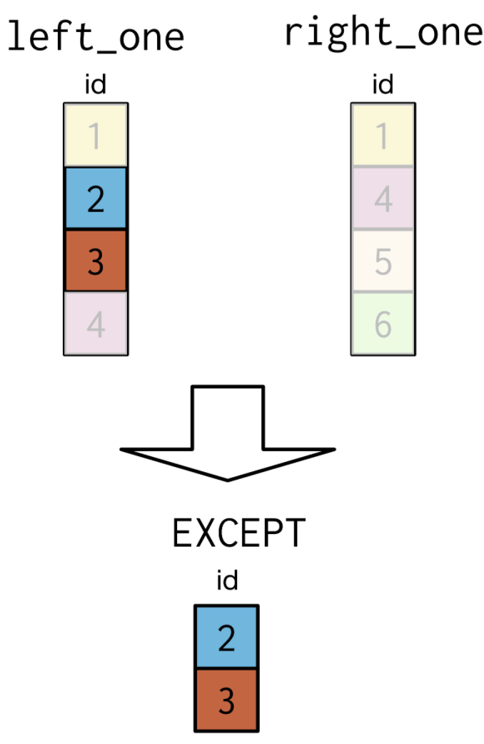
INTERSECT results in only those records found in both of the tables.
EXCEPT results in only those records in one table, BUT NOT the other.

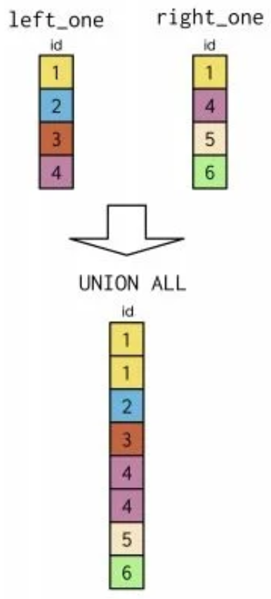
UNION does have no duplicate while UNION ALL includes all duplicates.

3.1.1. UNION & UNION ALL example¶

monarchs table in the leaders databAse Use UNION on the prime_ministers and monarchs tables all prime ministers and monarchs

Select prime_minister As leader,
country
From leaders.prime_ministers
UNION
Select monarch,
country
From leaders.monarchs
Order By country;

Note that the prime_minister field hAs been aliAsed As leader. The resulting field from the UNION will have the name leader.
- This is an important property of set theory clauses
The fields included in the operation must be of the same data type since they are returned As a single field.
- A number field can't be stacked on top of a character field.
Spain and Norway have a prime minister and a monarch, while Brunei and Oman have a monarch who also acts As a prime minister.

Select prime_minister As leader,
country
From leaders.prime_ministers
UNION ALL
Select monarch,
country
From leaders.monarchs
Order By country;

UNION and UNION ALL clauses do not do the lookup step that Joins do, they stack records on top of each other From one table to the next.

sql_stmt = "Select * \
From leaders.monarchs;"

pd.read_sql(sql_stmt, conn)

sql_stmt = "Select prime_minister As leader, \
                    country \
From leaders.prime_ministers \
UNION \
Select monarch, country \
From leaders.monarchs \
ORDER BY country;"

pd.read_sql(sql_stmt, conn)

sql_stmt = "Select prime_minister As leader, country \
From leaders.prime_ministers \
UNION ALL \
Select monarch, country \
From leaders.monarchs \
ORDER BY country;"

pd.read_sql(sql_stmt, conn)

3.1.2. Exercises¶

3.1.2.1. UNION¶

Near query result to the right, you will see two new tables with names economies2010 and economies2015.

Instructions

Combine these two tables into one table containing all of the fields in economies2010. The economies table is also included for reference.
Sort this resulting single table by country code and then by year, both in Ascending order.

Select *
From countries.economies2010
UNION
Select *
From countries.economies2015
Order By code, year;

sql_stmt = "\
Select * \
  From countries.economies2010 \
    UNION \
Select * \
  From countries.economies2015 \
ORDER BY code, year; \
"

pd.read_sql(sql_stmt, conn)

3.1.2.2. UNION (2)¶

UNION can also be used to determine all occurrences of a field across multiple tables. Try out this exercise with no starter code.

Instructions

Determine all (non-duplicated) country codes in either the cities or the currencies table. The result should be a table with only one field called country_code.
Sort by country_code in alphabetical order.

Select country_code
From countries.citie
UNION
Select code
From countries.currencies
Order By country_code;

sql_stmt = "\
Select country_code \
From countries.cities \
UNION \
Select code \
From countries.currencies \
Order BY country_code;"

country_codes = pd.read_sql(sql_stmt, conn)
country_codes.head()

country_codes.tail()

3.1.2.3. UNION ALL¶

As you saw, duplicates were removed From the previous two exercises by Using UNION. To include duplicates, you can use UNION ALL.

Instructions

Determine all combinations (include duplicates) of country code and year that exist in either the economies or the populations tables. Order by code then year.
The result of the query should only have two columns/fields. Think about how many records this query should result in.
You'll use code very similar to this in your next exercise after the video. Make note of this code after completing it.

Select code, year
From countries.economies
UNION All
Select country_code, year
From countries.populations
Order By code, year;

sql_stmt = "\
Select code, year \
  From countries.economies \
    UNION ALL \
Select country_code, year \
  From countries.populations \
ORDER BY code, year; \
"

country_codes_year = pd.read_sql(sql_stmt, conn)
country_codes_year.head()

country_codes_year.tail()

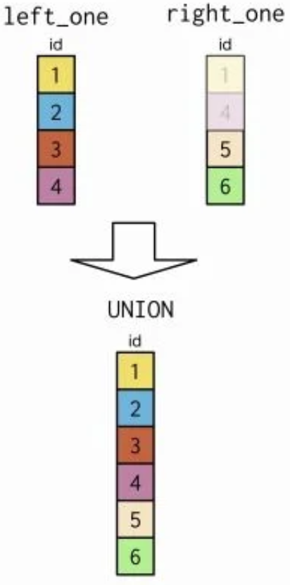
3.2. INTERSECT¶

Select id
From left_one
Intersect
Select id
From right_one;

The set theory clause INTERSECT works in a similar fAshion to UNION and UNION ALL, but remember From the Venn diagram, INTERSECT only includes those records in common to both tables and fields Selected.
The result only includes records common to the tables Selected
Determine countries with both a prime minister and president
The code for each of these set operations has a similar layout.
- First Select which fields to include From the first table, and then specify the name of the first table.
- Specify the set operation to perform
- Lastly, denote which fields to include From the second table, and then the name of the second table.

Select country
From leaders.prime_ministers
Intersect
Select country
From leaders.presidents;

What happens if two columns are Selected, instead of one?

Select country,
prime_minister As leader
From leaders.prime_ministers
Intersect
Select country, president
From leaders.presidents;

Will this also give you the names of the countries with both type of leaders?
This results in an empty table.
When INTERSECT looks at two columns, it includes both columns in the search.
- It didn't find any countries with prime ministers AND presidents having the same name.
- INTERSECT looks for records in common, not individual key fields like what a Join does to match.

sql_stmt = "\
Select country \
From leaders.prime_ministers \
INTERSECT \
Select country \
From leaders.presidents \
"

pd.read_sql(sql_stmt, conn)

3.2.1. Exercises¶

3.2.1.1. INTERSECT¶

Repeat the previous UNION ALL exercise, this time looking at the records in common for country code and year for the economies and populations tables.

Instructions

Again, order by code and then by year, both in Ascending order.
Note the number of records here (given at the bottom of query result) compared to the similar UNION ALL query result (814 records).

Select code, year
From countries.economies
INTERSECT
Select country_code, year
From countries.populations
Order By code, year;

sql_stmt = "\
Select code, year \
  From countries.economies \
    INTERSECT \
Select country_code, year \
  From countries.populations \
ORDER BY code, year; \
"

pd.read_sql(sql_stmt, conn)

3.2.1.2. INTERSECT (2)¶

As you think about major world cities and their corresponding country, you may Ask which countries also have a city with the same name As their country name?

Instructions

Use INTERSECT to answer this question with countries and cities!

sql_stmt = "\
Select name \
  From countries.countries \
    INTERSECT \
Select name \
  From countries.cities; \
"

pd.read_sql(sql_stmt, conn)

Hong Kong is part of China, but it appears separately here because it hAs its own ISO country code. Depending upon your analysis, treating Hong Kong separately could be useful or a mistake. Always check your datAset closely before you perform an analysis!

3.2.1.3. Review UNION and INTERSECT¶

Which of the following combinations of terms and definitions is correct?

Answer the question

~~UNION: returns all records (potentially duplicates) in both tables~~
~~UNION ALL: returns only unique records~~
INTERSECT: returns only records appearing in both tables</strong>

~~None of the above are matched correctly~~

3.3. EXCEPT¶

Select monarch, country
From leaders.monarchs
Intersect
Select prime_minister, country
From leaders.prime_ministers;

EXCEPT includes only the records in one table, but not in the other.
There are some monarchs that also act As the prime minister. One way to determine those monarchs in the monarchs table that do not also hold the title prime minister, is to use the EXCEPT clause.
This SQL query Selects the monarch field From monarchs, then looks for common entries with the prime_ministers field, while also keeping track of the country for each leader.
Only the two European monarchs are not also prime ministers in the leaders database.
Only the records that appear in the left table, BUT DO NOT appear in the right table are included.

sql_stmt = "\
Select monarch, country \
From leaders.monarchs \
EXCEPT \
Select prime_minister, country \
From leaders.prime_ministers; \
"

pd.read_sql(sql_stmt, conn)

3.3.1. Exercises¶

3.3.1.1. EXCEPT¶

Get the names of cities in cities which are not noted As capital cities in countries As a single field result.

Note that there are some countries in the world that are not included in the countries table, which will result in some cities not being labeled As capital cities when in fact they are.

Instructions

Order the resulting field in Ascending order.
Can you spot the city/cities that are actually capital cities which this query misses?

sql_stmt = "\
Select name \
  From countries.cities \
    EXCEPT \
Select capital \
  From countries.countries \
ORDER BY name; \
"

pd.read_sql(sql_stmt, conn).head()

3.3.1.2. EXCEPT (2)¶

Now you will complete the previous query in reverse!

Determine the names of capital cities that are not listed in the cities table.

Instructions

Order by capital in Ascending order.
The cities table contains information about 236 of the world's most populous cities. The result of your query may surprise you in terms of the number of capital cities that DO NOT appear in this list!

sql_stmt = "\
Select capital \
  From countries.countries \
    EXCEPT \
Select name \
  From countries.cities \
ORDER BY capital; \
"

pd.read_sql(sql_stmt, conn).head()

3.4. Semi-Joins and Anti-Joins¶

The previous six Joins are all additive Joins, in that they add columns to the original left table.
- Inner Join
- SELF Join
- LEFT Join
- RIGHT Join
- FULL Join
- CROSS Join
The lAst two Joins use a right table to determine which records to keep in the left table.
- Use these lAst to Joins in a way similar to a WHERE clause dependent on the values of a second table.
semi-Joins and anti-Joins don't have the same built-in SQL syntax that Inner Join and LEFT Join have.
semi-Joins and anti-Joins are useful tools in filtering table records on the records of another table.
The challenge will be to combine set theory clauses with semi-Joins.

3.4.1. SEMI Join¶

Determine the presidents of countries that gained independence before 1800.

Select president, country, continent
From leaders.presidents
Where country In
(Select name
From leaders.states
Where indep_year<1800);

This is an example of a subquery, which is a query that sits inside another query.

Does this include the presidents of Spain and Portugal?
- Since Spain does not have a president, it's not included here and only the Portuguese president is listed.
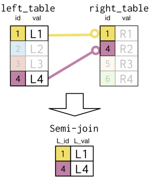
The semi-Join chooses records in the first table where a condition IS met in the second table.
The semi-Join matches records by key field in the right table with those in the left.
It then picks out only the rows in the left table that match the condition.

sql_stmt = "\
Select president, country, continent \
From leaders.presidents \
WHERE country IN \
    (Select name \
     From leaders.states \
     WHERE indep_year < 1800); \
"

pd.read_sql(sql_stmt, conn)

3.4.2. ANTI Join¶

Determine countries in the AmericAs founded after 1800.

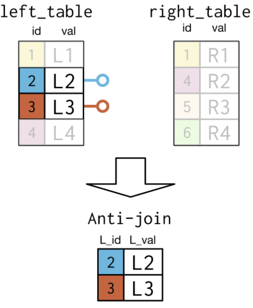
Select president, country, continent
From leaders.presidents
Where continent Like '%America'
And country Not In
(Select name
From leaders.states
Where indep_year<1800);

An anti-Join chooses records in the first table where a condition IS NOT met in the second table.
Use NOT to exclude those countries in the subquery.
The anti-Join picks out those columns in the left table that do not match the condition on the right table.

sql_stmt = "\
Select president, country, continent \
From leaders.presidents \
WHERE continent LIKE '%%America' \
    AND country NOT IN \
        (Select name \
         From leaders.states \
         WHERE indep_year < 1800); \
"

pd.read_sql(sql_stmt, conn)

3.4.3. Exercises¶

3.4.3.1. Semi-Join¶

You are now going to use the concept of a semi-Join to identify languages spoken in the Middle East.

Instructions 1)

Flash back to our Intro to SQL for Data Science course and begin by Selecting all country codes in the Middle EAst As a single field result Using Select, From, and Where.

sql_stmt = "\
Select code \
From countries.countries \
Where region = 'Middle East'; \
"

pd.read_sql(sql_stmt, conn)

You are now going to use the concept of a semi-Join to identify languages spoken in the Middle East.

Instructions 2)

Comment out the answer to the previous tab by surrounding it in /* and */. You'll come back to it!
Below the commented code, Select only unique languages by name appearing in the languages table.
Order the resulting single field table by name in Ascending order.

sql_stmt = "\
Select DISTINCT name \
From countries.languages \
ORDER BY name; \
"

pd.read_sql(sql_stmt, conn)

You are now going to use the concept of a semi-Join to identify languages spoken in the Middle East.

Instructions 3)

Now combine the previous two queries into one query:

Add a Where In statement to the Select Distinct query, and use the commented out query From the first instruction in there. That way, you can determine the unique languages spoken in the Middle EAst.

Carefully review this result and its code after completing it. It serves As a great example of subqueries, which are the focus of Chapter 4.

sql_stmt = "\
Select DISTINCT name \
From countries.languages \
Where code In \
 (Select code \
  From countries.countries \
  Where region = 'Middle East') \
Order BY name; \
"

pd.read_sql(sql_stmt, conn)

3.4.3.2. Relating semi-Join to a tweaked Inner Join<¶

Let's revisit the code From the previous exercise, which retrieves languages spoken in the Middle East.

Select Distinct name
From languages
Where code In
(Select name
From countries
Where region='Middle East')
Order By name;

Sometimes problems solved with semi-Joins can also be solved Using an Inner Join.

Select Distinct languages.name As language
From languages
Inner Join countries On languages.code = countries.code
Where region='Middle East')
Order By language;

This Inner Join isn't quite right. What is missing From this second code block to get it to match with the correct answer produced by the first block?

Possible Answers

~~HAVING instead of WHERE~~
DISTINCT</strong>

~~UNIQUE~~

sql_stmt = "\
Select DISTINCT languages.name As language \
From countries.languages \
Inner Join countries.countries \
On languages.code = countries.code \
Where region = 'Middle East' \
Order BY language;"

pd.read_sql(sql_stmt, conn)

3.4.3.3. Diagnosing problems Using anti-Join¶

Another powerful Join in SQL is the anti-Join. It is particularly useful in identifying which records are caUsing an incorrect number of records to appear in Join queries.

You will also see another example of a subquery here, As you saw in the first exercise on semi-Joins. Your goal is to identify the currencies used in Oceanian countries!

Instructions 1)

Begin by determining the number of countries in countries that are listed in Oceania Using Select, From, and WHERE.

sql_stmt = "\
Select count(name) \
From countries.countries \
Where continent = 'Oceania'; \
"

pd.read_sql(sql_stmt, conn)

Instructions 2)

Complete an Inner Join with countries As c1 on the left and currencies As c2 on the right to get the different currencies used in the countries of Oceania.
Match ON the code field in the two tables.
Include the country code, country name, and bAsic_unit As currency.

Observe query result and make note of how many different countries are listed here.

sql_stmt = "\
Select c1.code, \
        c1.name, \
        c2.bAsic_unit As currency \
From countries.countries As c1 \
Inner Join countries.currencies As c2 \
On c1.code = c2.code \
Where continent = 'Oceania'; \
"

pd.read_sql(sql_stmt, conn)

Instructions 3)

Note that not all countries in Oceania were listed in the resulting Inner Join with currencies. Use an anti-Join to determine which countries were not included!

Use NOT IN and (Select code From currencies) As a subquery to get the country code and country name for the Oceanian countries that are not included in the currencies table.

sql_stmt = "\
Select code, name \
  From countries.countries \
  WHERE continent = 'Oceania' \
    AND code NOT IN \
    (Select code \
     From countries.currencies); \
"

pd.read_sql(sql_stmt, conn)

3.4.3.4. Set theory challenge¶

Congratulations! You've now made your way to the challenge problem for this third chapter. Your tAsk here will be to incorporate two of UNION/UNION ALL/INTERSECT/EXCEPT to solve a challenge involving three tables.

In addition, you will use a subquery As you have in the lAst two exercises! This will be great practice As you hop into subqueries more in Chapter 4!

Instructions

Identify the country codes that are included in either economies or currencies but not in populations.
Use that result to determine the names of cities in the countries that match the specification in the previous instruction.

sql_stmt = "\
Select country_code, name \
From countries.cities As c1 \
Where country_code In \
    (Select e.code \
     From countries.economies As e \
     UNION ALL \
     Select c2.code \
     From countries.currencies As c2 \
     EXCEPT \
     Select p.country_code \
     From countries.populations As p); \
"

pd.read_sql(sql_stmt, conn)

4. Subqueries¶

In this closing chapter, you'll learn how to use nested queries to add some finesse to your data insights. You'll also wrap all of the content covered throughout this course into solving three challenge problems.

4.1. Subqueries inside WHERE and Select clauses¶

The most common type of subquery is one inside of a WHERE statement.
- Examples include semi-Join and anti-Join

sql_stmt = "\
Select name, fert_rate \
From leaders.states \
Where continent = 'Asia' \
And fert_rate <  \
(Select AVG(fert_rate) \
 From leaders.states); \
"

pd.read_sql(sql_stmt, conn)

The second most common type of subquery is inside of a Select clause.

Count the number of countries listed in states table for each continent in the prime_ministers table.

Continents in the prime_ministers table

Determine the counts of the number of countries in states for each of the continents in the lAst slide

Select count(name)
From leaders.states
Where continent In
(Select Distinct continent
From leaders.prime_ministers);
-- From languages

Select Distinct continent,
(Select Count(*)
From leaders.states
Where prime_ministers.continent = states.continent) As countries_num
From leaders.prime_ministers;

The subquery involving states, can also reference the prime_ministers table in the main query.
Anytime you do a subquery inside a Select statement, you need to give the subquery an aliAs (e.g. countries_num in the example)
There are numerous ways to solve problems with SQL queries. A carefully constructed Join could achieve this same result.

sql_stmt = "\
Select DISTINCT continent, \
            (Select COUNT(*) \
             From leaders.states \
             Where prime_ministers.continent = states.continent) As countries_num \
From leaders.prime_ministers \
"

pd.read_sql(sql_stmt, conn)

4.1.1. Exercises¶

4.1.1.1. Subquery inside WHERE¶

You'll now try to figure out which countries had high average life expectancies (at the country level) in 2015.

Instructions 1)

Begin by calculating the average life expectancy across all countries for 2015.

sql_stmt = "\
Select avg(life_expectancy) \
  From countries.populations \
Where year = 2015; \
"

pd.read_sql(sql_stmt, conn)

Instructions 2)

Recall that you can use SQL to do calculations for you. Suppose we wanted only records that were above 1.15 * 100 in terms of life expectancy for 2015:
Select *,
From populations
Where life_expectancy>1.15*100 And year=2015;

Select all fields From populations with records corresponding to larger than 1.15 times the average you calculated in the first tAsk for 2015. In other words, change the 100 in the example above with a subquery.

sql_stmt = "\
Select * \
From countries.populations \
Where life_expectancy > 1.15 * \
           (Select avg(life_expectancy) \
           From countries.populations \
           Where year = 2015) And year = 2015; \
"

pd.read_sql(sql_stmt, conn)

4.1.1.2. Subquery inside WHERE (2)¶

Use your knowledge of subqueries in Where to get the urban area population for only capital cities.

Instructions

Make use of the capital field in the countries table in your subquery.
Select the city name, country code, and urban area population fields.

sql_stmt = "\
Select name, country_code, urbanarea_pop \
  From countries.cities \
Where name In \
  (Select capital \
   From countries.countries) \
Order BY urbanarea_pop Desc; \
"

pd.read_sql(sql_stmt, conn)

4.1.1.3 Subquery inside Select¶

In this exercise, you'll see how some queries can be written Using either a Join or a subquery.

You have seen previously how to use GROUP BY with aggregate functions and an Inner Join to get summarized information From multiple tables.

The code given in query.sql Selects the top nine countries in terms of number of cities appearing in the cities table. Recall that this corresponds to the most populous cities in the world. Your tAsk will be to convert the commented out code to get the same result As the code shown.

Instructions 1)

Submit your Answer:

sql_stmt = "\
Select countries.name As country, \
        COUNT(*) As cities_num \
From countries.cities \
Inner Join countries.countries \
On countries.code = cities.country_code \
Group BY country \
Order BY cities_num Desc, country \
LIMIT 9; \
"

pd.read_sql(sql_stmt, conn)

Instructions 2)

Remove the comments around the second query and comment out the first query instead.
Convert the GROUP BY code to use a subquery inside of Select, i.e. fill in the blanks to get a result that matches the one given Using the GROUP BY code in the first query.
Again, sort the result by cities_num descending and then by country Ascending.

sql_stmt = "\
Select countries.name As country, \
      (Select count(*) \
       From countries.cities \
       Where countries.code = cities.country_code) As cities_num \
From countries.countries \
Order BY cities_num Desc, country \
LIMIT 9; \
"

pd.read_sql(sql_stmt, conn)

4.2. Subquery inside From clause¶

The last basic type of subquery exists inside of a From clause. Determine the maximum percentage of women in parliament for each continent listing in leaders.states

Select continent,
Max(women_parli_perc) As max_perc
From states
Group By continent
Order By continent;

This query will only work if continent is included As one of th fields in the Select clause, since we are grouping bAsed on that field.

sql_stmt = "\
Select continent, MAX(women_parli_perc) As max_perc \
From leaders.states \
Group BY continent \
Order BY continent; \
"

pd.read_sql(sql_stmt, conn)

FocUsing on records in monarchs

Multiple tables can be included in the From clause, by adding a comma between them
Produces part of the answer; how should duplicates be removed?

sql_stmt = "\
Select monarchs.continent \
From leaders.monarchs, leaders.states \
Where monarchs.continent = states.continent \
Order BY continent; \
"

pd.read_sql(sql_stmt, conn)

Finishing the subquery

To get Asia and Europe to appear only once, use DISTINCT in the Select statement.
How is the max_perc column included with continent? Instead of including states in the From clause, include the subquery instead and aliAs it with a name like subquery.
This is how to include a subquery As a temporary table in the From clause.

sql_stmt = "\
Select DISTINCT monarchs.continent, subquery.max_perc \
From leaders.monarchs, \
    (Select continent, MAX(women_parli_perc) As max_perc \
     From leaders.states \
     GROUP BY continent) As subquery \
WHere monarchs.continent = subquery.continent \
Order BY continent; \
"

pd.read_sql(sql_stmt, conn)

4.2.1. Exercises¶

4.2.1.1. Subquery inside From¶

The last type of subquery you will work with is one inside of From.

You will use this to determine the number of languages spoken for each country, identified by the country's local name! (Note this may be different than the name field and is stored in the local_name field.)

Instructions 1)

Begin by determining for each country code how many languages are listed in the languages table using Select, From, and GROUP BY. Alias the aggregated field As lang_num.

sql_stmt = "\
Select code, count(name) As lang_num \
From countries.languages \
GROUP BY code \
ORDER BY lang_num DESC; \
"

lang_count = pd.read_sql(sql_stmt, conn)
print(lang_count.head())
print(lang_count.tail())

  code  lang_num
0  ZMB        19
1  ZWE        16
2  ETH        16
3  IND        14
4  NPL        14
    code  lang_num
207  COL         1
208  AIA         1
209  DOM         1
210  SAU         1
211  PRK         1

Instructions 2)

Include the previous query (aliAsed As subquery) As a subquery in the From clause of a new query.
Select the local name of the country From countries.
Also, Select lang_num From subquery.
Make sure to use WHERE appropriately to match code in countries and in subquery.
Sort by lang_num in descending order.

sql_stmt = "\
Select local_name, \
        subquery.lang_num \
From countries.countries, \
        (Select code, count(name) As lang_num \
         From countries.languages \
         Group BY code) As subquery \
         Where countries.code = subquery.code \
Order BY lang_num DESC; \
"

lang_count = pd.read_sql(sql_stmt, conn)
print(lang_count.head())
print(lang_count.tail())

     local_name  lang_num
0        Zambia        19
1   YeItyop´iya        16
2      Zimbabwe        16
3  Bharat/India        14
4         Nepal        14
                       local_name  lang_num
194          Republica Dominicana         1
195  The Turks and Caicos Islands         1
196                     Nederland         1
197                United Kingdom         1
198                        Brasil         1

4.2.1.2. Advanced subquery¶

You can also nest multiple subqueries to answer even more specific questions. In this exercise, for each of the six continents listed in 2015, you'll identify which country had the maximum inflation rate (and how high it was) Using multiple subqueries. The table result of your query in Task 3 should look something like the following, where anything between < > will be filled in with appropriate values:

name	continent	inflation_rate
<country1>	North America	<max_inflation1>
<country2>	Africa	<max_inflation2>
<country3>	Oceania	<max_inflation3>
<country4>	Europe	<max_inflation4>
<country5>	South America	<max_inflation5>
<country6>	Asia	<max_inflation6>

</code></pre> Again, there are multiple ways to get to this solution Using only Joins, but the focus here is on showing you an introduction into advanced subqueries.

Instructions 1)

Create an Inner Join with countries on the left and economies on the right with Using. Do not alias your tables or columns.
Retrieve the country name, continent, and inflation rate for 2015.

sql_stmt = "\
Select name, continent, inflation_rate \
  From countries.countries \
    Inner Join countries.economies \
    Using (code) \
WHERE year = 2015; \
"

inf_rate = pd.read_sql(sql_stmt, conn)
print(inf_rate.head())
print(inf_rate.tail())

                   name      continent  inflation_rate
0           Afghanistan           Asia          -1.549
1                Angola         Africa          10.287
2               Albania         Europe           1.896
3  United Arab Emirates           Asia           4.070
4             Argentina  South America             NaN
             name continent  inflation_rate
180         Samoa   Oceania           1.923
181         Yemen      Asia          39.403
182  South Africa    Africa           4.575
183        Zambia    Africa          10.107
184      Zimbabwe    Africa          -2.410

Instructions 2)

Determine the maximum inflation rate for each continent in 2015 Using the previous query As a subquery called subquery in the From clause.
Select the maximum inflation rate As max_inf grouped by continent.
This will result in the six maximum inflation rates in 2015 for the six continents as one field table. (Don't include continent in the outer Select statement.)

sql_stmt = "\
Select max(inflation_rate) As max_inf \
  From ( \
      Select name, continent, inflation_rate \
      From countries.countries \
      Inner Join countries.economies \
      Using (code) \
      WHERE year = 2015) As subquery \
GROUP BY continent; \
"

pd.read_sql(sql_stmt, conn)

Instructions 3)

Append the second part's query to the first part's query using Where, And, and In to obtain the name of the country, its continent, and the maximum inflation rate for each continent in 2015. Revisit the sample output in the Assignment text at the beginning of the exercise to see how this matches up.
For the sake of practice, change all Joining conditions to use On instead of Using.
This code works since each of the six maximum inflation rate values occur only once in the 2015 data. Think about whether this particular code involving subqueries would work in cAses where there are ties for the maximum inflation rate values.

sql_stmt = "\
Select name, continent, inflation_rate \
  From countries.countries \
    Inner Join countries.economies \
    ON countries.code = economies.code \
  WHERE year = 2015 \
    AND inflation_rate IN ( \
         Select max(inflation_rate) As max_inf \
         From ( \
               Select name, continent, inflation_rate \
               From countries.countries \
               Inner Join countries.economies \
               ON countries.code = economies.code \
               WHERE year = 2015) As subquery \
        GROUP BY continent); \
"

pd.read_sql(sql_stmt, conn)

4.2.1.3. Subquery challenge¶

Let's test your understanding of the subqueries with a challenge problem! Use a subquery to get 2015 economic data for countries that do not have

gov_form of 'Constitutional Monarchy' or
'Republic' in their gov_form.

Here, gov_form stands for the form of the government for each country. Review the different entries for gov_form in the countries table.

Instructions

Select the country code, inflation rate, and unemployment rate.
Order by inflation rate Ascending.
Do not use table aliAsing in this exercise.

-- Select fields
Select code,
inflation_rate,
unemployment_rate
-- From economies
From economies
-- Where year is 2015 and code is not in
Where year=2015 And code Not In
-- Subquery of the codes that gov_form is 'Constitutional Monarchy' or '%Republic'
(Select code
From countries
Where (gov_form='Constitutional Monarchy' Or gov_form Like '%Republic'))
-- Order by inflation rate
Order By inflation_rate;

sql_stmt = "\
Select code, inflation_rate, unemployment_rate \
From countries.economies \
Where year = 2015 Ans code Not In \
    (Select code \
     From countries.countries \
     Where (gov_form = 'Constitutional Monarchy' Or gov_form Like '%%Republic')) \
Order BY inflation_rate; \
"

pd.read_sql(sql_stmt, conn)

4.2.1.4. Subquery review¶

Within which SQL clause are subqueries most frequently found?

Answer the question

Where</strong>

~~From~~

~~Select~~

IN

4.3. Course Review¶

In SQL, a Join combines columns From one or more tables in a relational databAse via a lookup process.
There are four types of Joins covered in this course

Types of Joins:

Inner Join: also denoted As Join
- Self-Joins: special cAse
OUTER Join
- LEFT Join: also denoted As LEFT OUTER Join
- RIGHT Join: also denoted As RIGHT OUTER Join
- FULL Join: also denoted As FULL OUTER Join
CROSS Join: create all possible combinations between two tables
Semi-Join / Anti-Join

Notes

Words appearing in ALL capital letters correspond to Joins having simple SQL syntax. Self-Joins, semi-Joins, and anti-Joins don't have built-in SQL syntax.

An Inner Join keeps only the records in which the key field (or fields) is in both tables. A LEFT Join keeps all the records in fields specified in the left table and includes the matches in the right table bAsed on the key field or fields. Key field values that don't match in the right table are included As missing data in the resulting table of a LEFT Join.

A RIGHT Join keeps all the records specified in the right table and includes the matches From the key field(s) in the left table. THose that don't match are included As missing values in the resulting table From the RIGHT Join query.

A FULL Join is a combination of a LEFT Join and a RIGHT Join showing exactly which values appear in both tables and those that appear in only one or the other table. A CROSS Join matches all records From fields specified in one table with all records From fields specified in another table. Remember that a CROSS Join does not have an On or Using clause, but otherwise looks very similar to the code for an Inner Join, LEFT Join, RIGHT Join, or FULL Join.

Set Theory Clauses

Recall that UNION includes every record in both tables but DOES NOT double count those that are in both tables.
UNION ALL does replicate those that are in both tables.
INTERSECT gives only those records found in both of the two tables.
EXCEPT gives only those records in one table but not the other.

Semi-Joins and Anti-Joins

When you'd like to filter your first table bAsed on conditions set on a second table, you should use a semi-Join to accomplish the tAsk.
If instead you'd like to filter the first table bAsed on conditions NOT being met on a second table, you should use an anti-Join.
- Anti-Joins are particularly useful in diagnosing problems with other Joins in terms of getting fewer or more records than expected.

Types of basic subqueries

The most common type of subquery is done inside of a WHERE clause.
The next most frequent types of subqueries are inside Select clauses and inside From clauses.
Subqueries can also find their way into the ON statement of a Join in ways similar to what you've seen inside WHERE clauses too.

4.3.1. Final Challenge¶

Welcome to the end of the course! The next three exercises will test your knowledge of the content covered in this course and apply many of the ideAs you've seen to difficult problems. Good luck!

Read carefully over the instructions and solve them step-by-step, thinking about how the different clauses work together. In this exercise, you'll need to get the country names and other 2015 data in the economies table and the countries table for Central American countries with an official language.

Instructions

Select unique country names. Also Select the total investment and imports fields.
Use a left Join with countries on the left. (An Inner Join would also work, but pleAse use a left Join here.)
Match on code in the two tables And use a subquery inside of On to choose the appropriate languages records.
Order by country name ascending.
Use table aliAsing but not field aliAsing in this exercise.

-- Select fields
Select Distinct c.name,
e.total_investment,
e.imports
-- From countries (with alias as c)
From countries As c
-- Join to economies (with alias as e
Left Join economies As e
-- Match on code in (c,e) and the c.code in official languages
On (c.code=e.code
And c.code In (Select l.code
From languages As l
Where official='true'))
-- Where region and year are correct
Where year=2015 And region='Central America'
-- Order by field
Order By name;

sql_stmt = "\
Select DISTINCT c.name, \
                e.total_investment, \
                e.imports \
From countries.countries As c \
LEFT Join countries.economies As e \
On (c.code = e.code \
                And c.code IN (Select l.code \
                              From countries.languages As l \
                              Where official = 'true'))\
Where year = 2015 And region = 'Central America' \
Order BY name; \
"

pd.read_sql(sql_stmt, conn)

4.3.2. Final Challenge (2)¶

Let's ease up a bit and calculate the average fertility rate for each region in 2015.

Instructions

Include the name of region, its continent, and average fertility rate aliAsed As avg_fert_rate.
Sort bAsed on avg_fert_rate ascending.
Remember that you'll need to Group BY all fields that aren't included in the aggregate function of Select.

-- Select fields
Select c.name,
c.continent,
Avg(p.fertility_rate) As avg_fert_rate
-- From populations (with alias as p)
From populations As p
-- Join to countries (with alias as c
Inner Join countries As c
-- Match on code in (p,c)
On p.country_code=c.code
Where year=2015
-- Group by continent and region
Group By c.continent, c.region
-- Order by avg of fertility_rate
Order By avg_fert_rate;

sql_stmt = "\
Select c.region, \
       c.continent, \
       AVG(p.fertility_rate) As avg_fert_rate \
From countries.populations As p \
Inner Join countries.countries As c \
ON p.country_code = c.code \
Where year = 2015 \
Group BY c.continent, c.region \
Order BY avg_fert_rate; \
"

pd.read_sql(sql_stmt, conn)

4.3.3. Final Challenge (3)¶

Welcome to the lAst challenge problem. Remember that these challenges are designed to take you to the limit to solidify your SQL knowledge! Take a deep breath and solve this step-by-step.

You are now tAsked with determining the top 10 capital cities in Europe and the AmericAs in terms of a calculated percentage using city_proper_pop and metroarea_pop in cities. Do not use table aliAsing in this exercise.

Instructions

Select the city name, country code, city proper population, and metro area population.
Calculate the percentage of metro area population composed of city proper population for each city in cities, aliased as city_perc.
Focus only on capital cities in Europe and the Americas in a subquery.
Make sure to exclude records with missing data on metro area population.
Order the result by city_perc descending.
Then determine the top 10 capital cities in Europe and the Americas in terms of this city_perc percentage.

-- Select fields
Select name,
country_code,
city_proper_pop,
metroarea_pop,
-- Calculate city_perc
city_proper_pop/metroarea_pop*100 As city_perc
-- From cities
From cities
-- Where the names from continent='Europe' or '%America' and metroarea_pop is not null
Where name In
(Select capital
From countries
Where (continent='Europe' Or continent Like '%America'))
And metroarea_pop Is Not Null
-- Order by city_perc in descreasing order
Order By city_perc Desc
Limit 10;

sql_stmt = "\
Select name, \
       country_code, \
       city_proper_pop, \
       metroarea_pop, \
       city_proper_pop / metroarea_pop * 100 As city_perc \
From countries.cities \
Where name In \
            (Select capital \
             From countries.countries \
             Where (continent = 'Europe' OR continent Like '%%America')) \
                       And metroarea_pop IS NOT NULL \
Order BY city_perc desc \
Limit 10; \
"

pd.read_sql(sql_stmt, conn)

# close the connection
conn.close()

Intermediate SQL Using SQLite¶

Course: DataCamp: Intermediate SQL Notebook Author: Jae Choi

Course Description

The European Soccer Database contains data about 12,800 matches from 11 countries played between 2011-2015! Throughout this course, you will be shown filtered versions of the tables in this database in order to better explore their contents.

You’ve learned how to Joining Data in SQL from tables

This course will teach you to wrangle, filter, and categorize information in a relational database.
Learn the robust use of CASE statements, subqueries, and window functions
By discovering some interesting facts about soccer using the European Soccer Database.

Datasets

European Soccer Database

Imports

import sqlite3
path = "/Users/Jae/Google_Drive_jae0325/DATA_SCIENCE/Portfolio/datacamp/"
database = path + 'database.sqlite'
# Unix/Mac - 4 initial slashes in total (3+1 in front of database)
#engine = create_engine("sqlite:///"+database)

conn = sqlite3.connect(database)
table_stmt = """SELECT *
              FROM sqlite_master
              WHERE type='table';"""
tables = pd.read_sql(table_stmt, conn)
tables

1. CASE Statement¶

Learn how to use the CASE WHEN statement to create categorical variables, aggregate data into a single column with multiple filtering conditions, and calculate counts and percentages.

1.1. Basic CASE Usage¶

CASE Statement Introduction

Contains a WHEN, THEN, and ELSE statement, finished with END.
- Using AND to add multiple logical conditions to your WHEN clause.
- If there is no ELSE, those don’t meet the conditions are NULL
CASE statements are great for…
- Categorizing data
- Filtering data with WHERE
- Aggregating data
CASE statements will return any value you specify in your THEN clause.
- This is an incredibly powerful tool for robust calculations and data manipulation when used in conjunction with an aggregate statement.
- One key task you can perform is using CASE inside an AVG function to calculate a percentage of information in your database.

1.1.1. Example: Basic `CASE` Statement¶

In this exercise, you will identify matches played between FC Schalke 04 and FC Bayern Munich.

sql_stmt="""-- Identify the home team as Bayern Munich, Schalke 04, or neither
SELECT 
    CASE WHEN home_team_api_id = 10189 THEN 'FC Schalke 04'
         WHEN home_team_api_id = 9823 THEN 'FC Bayern Munich'
         ELSE 'Other' END AS home_team,
    COUNT(id) AS total_matches
FROM Match
WHERE country_id = 7809 -- Germany
-- Group by the CASE statement alias
GROUP BY home_team;
"""
pd.read_sql(sql_stmt, conn)

1.2. Complex `CASE` Statement¶

CASE & Alias

Remember, just like subqueries, you don’t need alias statement inside WHERE.
But you need alias statement inside SELECT, FROM.

1.2.1. Example: `CASE` Statements Inside `SELECT`, Comparing Column Values¶

Barcelona is considered one of the strongest teams in Spain's soccer league.

You will be creating a list of matches in the 2011/2012 season where Barcelona was the "home team". You will do this using a CASE statement that compares the values of two columns to create a new group -- wins, losses, and ties.

sql_stmt = """SELECT
    m.date,
    t.team_long_name AS opponent,
    -- Complete the CASE statement with an alias
    CASE WHEN m.home_team_goal > m.away_team_goal THEN 'Barcelona win!'
        WHEN m.home_team_goal < m.away_team_goal THEN 'Barcelona loss :(' 
        ELSE 'Tie' END AS outcome 
FROM Match AS m
LEFT JOIN Team AS t 
ON m.away_team_api_id = t.team_api_id
-- Filter for Barcelona as the home team
WHERE m.home_team_api_id = 8634
  AND season = '2011/2012';"""
pd.read_sql(sql_stmt, conn).head()

Now, construct a query to determine the outcome of Barcelona's matches where they played as the "away team". Did their performance differ from the matches where they were the home team?

sql_stmt = """-- Select matches where Barcelona was the away team
SELECT  
    m.date,
    t.team_long_name AS opponent,
    CASE WHEN m.home_team_goal < m.away_team_goal THEN 'Barcelona win!'
        WHEN m.home_team_goal > m.away_team_goal THEN 'Barcelona loss :(' 
        ELSE 'Tie' END AS outcome
FROM Match AS m
-- Join teams_spain to matches_spain
LEFT JOIN Team AS t 
ON m.home_team_api_id = t.team_api_id
WHERE m.away_team_api_id = 8634
  AND season = '2011/2012';"""
pd.read_sql(sql_stmt, conn).head()

Barcelona's performance seems to be worse when they are the away team.

1.2.2. Example: Filtering with `CASE` Statement Inside `WHERE`¶

Generate a list of matches won by Italy's Bologna team!

sql_stmt = """-- Select the season, date, home_goal, and away_goal columns
SELECT 
    season,
    date,
    home_team_goal,
    away_team_goal
FROM Match
WHERE 
-- Exclude games not won by Bologna
    CASE WHEN home_team_api_id = 9857 AND home_team_goal > away_team_goal THEN 'Bologna Win'
        WHEN away_team_api_id = 9857 AND away_team_goal > home_team_goal THEN 'Bologna Win' 
        END IS NOT NULL;"""
pd.read_sql(sql_stmt, conn).head()

You now have details on every match in this database where Bologna won.

1.3. `CASE` with Aggregation¶

CASE with Aggregation Functions -CASE WHEN with COUNT(): Count the rows. -CASE WHEN with SUM(): Sum the values. -CASE WHEN with AVG(): Average of values, or calculate percentage.

1.3.1. Example: `COUNT` using `CASE WHEN`¶

Do the number of soccer matches played in a given European country differ across seasons?

sql_stmt = """SELECT 
    c.name AS country,
    -- Count matches in each of the 3 seasons
    COUNT(CASE WHEN m.season = '2012/2013' THEN m.id END) AS matches_2012_2013,
    COUNT(CASE WHEN m.season = '2013/2014' THEN m.id END) AS matches_2013_2014,
    COUNT(CASE WHEN m.season = '2014/2015' THEN m.id END) AS matches_2014_2015
FROM country AS c
LEFT JOIN match AS m
ON c.id = m.country_id
-- Group by country name alias
GROUP BY country;"""
pd.read_sql(sql_stmt, conn).head()

The number of matches played in each season seems relatively consistent across countries. Where do you see the largest difference?

1.3.2. Example: `SUM` and `CASE WHEN` with Multiple Conditions¶

In Python, you have the ability to calculate a SUM of logical values (i.e., TRUE/FALSE) directly. In SQL, you have to convert these values into 1 and 0 before calculating a sum. This can be done using a CASE statement.

Your goal here is to use the country and match table to determine the total number of matches won by the home team in each country during the different seasons.

sql_stmt = """SELECT 
    c.name AS country,
    -- Sum the total records in each season where the home team won
    SUM(CASE WHEN m.season = '2012/2013' AND m.home_team_goal > m.away_team_goal 
        THEN 1 ELSE 0 END) AS matches_2012_2013,
    SUM(CASE WHEN m.season = '2013/2014' AND m.home_team_goal > m.away_team_goal 
        THEN 1 ELSE 0 END) AS matches_2013_2014,
    SUM(CASE WHEN m.season = '2014/2015' AND m.home_team_goal > m.away_team_goal 
        THEN 1 ELSE 0 END) AS matches_2014_2015
FROM country AS c
LEFT JOIN match AS m
ON c.id = m.country_id
-- Group by country name alias
GROUP BY country;
"""
pd.read_sql(sql_stmt, conn).head()

1.3.2. Example: Calculating Percent with `CASE` and `AVG`¶

Examine the percentage of ties in each country in different seasons.

sql_stmt = """SELECT 
    c.name AS country,
    -- Round the percentage of tied games to 2 decimal points
    -- Calculate the percentage of tied games in each season
    ROUND(AVG(CASE WHEN m.season='2013/2014' AND m.home_team_goal = m.away_team_goal THEN 1
             WHEN m.season='2013/2014' AND m.home_team_goal != m.away_team_goal THEN 0
             END),2) AS pct_ties_2013_2014,
    ROUND(AVG(CASE WHEN m.season='2014/2015' AND m.home_team_goal = m.away_team_goal THEN 1
             WHEN m.season='2014/2015' AND m.home_team_goal != m.away_team_goal THEN 0
             END),2) AS pct_ties_2014_2015
FROM country AS c
LEFT JOIN match AS m
ON c.id = m.country_id
GROUP BY country;
"""
pd.read_sql(sql_stmt, conn).head()

2. Simple Subquery¶

Learn about subqueries in the SELECT, FROM, and WHERE clauses. You will gain an understanding of when subqueries are necessary to construct your dataset and where to best include them in your queries.

2.1. Subqueries in `WHERE`¶

What is a Subquery?

A query nested inside another query.
Useful for intermediary transformations.
Can be in any part of a query: SELECT, FROM, WHERE, GROUP BY.
Can return a variety of information
- Scalar quantities (Numbers).
- A list used for filtering or joining.
- A table to extract further transformation data.

Why Subqueries?

Comparing groups to summarized values.
- Eg. How did Liverpool compare to the English Premier League’s average performance for that year?
Reshaping data.
- Eg. What is the highest monthly average of goals scored in the Bundesliga?
Combining data that cannot be joined.
- Eg. How do you get both the home and away team names into a table of match results?

Subqueries in WHERE

Used for filtering results.
Subquery can be evaluated independently from the outer query.
Is only processed once in the entire statement.

2.1.1. Example: Filtering Using Scalar `WHERE` Subqueries¶

Generate a list of matches where the total goals scored (for both teams in total) is more than 3 times the average for games in the 2013/2014 matches.

sql_stmt = """SELECT 
    -- Select the date, home goals, and away goals scored
    date,
    home_team_goal,
    away_team_goal
FROM  match
-- Filter for matches where total goals exceeds 3x the average
WHERE season = '2013/2014' AND
      (home_team_goal + away_team_goal) > 
      (SELECT 3 * AVG(home_team_goal + away_team_goal)
        FROM match WHERE season = '2013/2014'); 
"""
pd.read_sql(sql_stmt, conn)

2.1.2. Example: Filtering Using `WHERE` Subqueries with a List¶

Create a list of teams that scored 8 or more goals in a home match.

sql_stmt = """SELECT
    -- Select the team long and short names
    team_long_name,
    team_short_name
FROM team
-- Filter for teams with 8 or more home goals
WHERE team_api_id IN
      (SELECT home_team_api_id 
       FROM match
       WHERE home_team_goal >= 8);
"""
pd.read_sql(sql_stmt, conn)

2.2. Subqueries in `FROM`¶

Subqueries in FROM

Restructure and transform your data
- Transforming data from long to wide before selecting
- Prefiltering data
Calculating aggregates of aggregates
- Eg. Which 3 teams has the highest average of home goals scored?
You can create multiple subqueries in one FROM statement
- Alias, and Join them!
You can join a subquery to a table in FROM
- Include a joining columns in both tables

2.2.1 Example: Joining Subqueries in `FROM`¶

Generate a subquery using the match table, and then join that subquery to the country table to calculate information about matches with 10 or more goals in total.

sql_stmt = """SELECT
    -- Select country name and the count match IDs
    c.name AS country_name,
    COUNT(sub.id) AS matches
FROM country AS c
-- Inner join the subquery onto country
-- Select the country id and match id columns
INNER JOIN (SELECT country_id, id 
           FROM match
           -- Filter the subquery by matches with 10+ goals
           WHERE (home_team_goal + away_team_goal) >= 10) AS sub
ON c.id = sub.country_id
GROUP BY country_name;
"""
pd.read_sql(sql_stmt, conn)

2.3. Subqueries in `SELECT`¶

Subqueries in SELECT

Returns a single value
- Include aggregate values to compare to individual values
- Used in mathematical calculations
Make sure you have all filters in the right places
- Properly filter both the main and the subquery!

2.3.1. Example: Subqueries in `SELECT` for Calculations¶

Create a column to compare each league's average total goals to the overall average goals in the 2013/2014 season. Also, add a column that directly compares these values by subtracting the overall average from the subquery.

sql_stmt = """SELECT
    -- Select the league name and average goals scored
    name AS league,
    ROUND(AVG(m.home_team_goal + m.away_team_goal),2) AS avg_goals,
    -- Subtract the overall average from the league average
    ROUND(AVG(m.home_team_goal + m.away_team_goal) - 
        (SELECT AVG(home_team_goal + away_team_goal)
         FROM match 
         WHERE season = '2013/2014'),2) AS diff
FROM league AS l
LEFT JOIN match AS m
ON l.country_id = m.country_id
-- Only include 2013/2014 results
WHERE season = '2013/2014'
GROUP BY league
ORDER BY avg_goals DESC;
"""
pd.read_sql(sql_stmt, conn)

Games in the Netherlands tend to score the highest number of goals on average in this season.

2.4. Subqueries Advice¶

Must Know When Using Subqueries

Can include multiple subqueries in SELECT, FROM, WHERE
Format your queries
- Line up SELECT, FROM, WHERE, and GROUP BY
Annotate your queries
- Comment: / ~ /
- In line Comment: -- ~
Indent your queries
- CASE WHEN statement
- Subqueries
Properly filter each subquery
Is that subquery necessary?
- Subqueries require computing power

2.4.1. Example: Subqueries Everywhere¶

In soccer leagues, games are played at different stages. Winning teams progress from one stage to the next, until they reach the final stage. In each stage, the stakes become higher than the previous one.

Extract data examining the average goals scored in each stage of a match. Does the average number of goals scored change as the stakes get higher from one stage to the next?

sql_stmt = """SELECT 
    -- Select the stage and average goals from s
    stage,
    ROUND(avg_goals,2) AS avg_goal,
    -- Select the overall average for 2012/2013
    ROUND((SELECT AVG(home_team_goal + away_team_goal) FROM match WHERE season = '2012/2013'),2) AS overall_avg
FROM 
    -- Select the stage and average goals in 2012/2013 from match
    (SELECT
         stage,
         AVG(home_team_goal + away_team_goal) AS avg_goals
     FROM match
     WHERE season = '2012/2013'
     GROUP BY stage) AS s
WHERE 
    -- Filter the main query using the subquery
    s.avg_goals > (SELECT AVG(home_team_goal + away_team_goal) 
                    FROM match WHERE season = '2012/2013')
ORDER BY stage DESC;
"""
pd.read_sql(sql_stmt, conn).head()

You used 3 subqueries to generate a list of stages that have higher than average goals scored in matches.

3. Advanced Subquery¶

Learn how to use nested and correlated subqueries to extract more complex data from a relational database. You will also learn about common table expressions and how to best construct queries using multiple common table expressions.

3.1. Correlated Subquery¶

Correlated Subquery

Uses values from the outer query to generate a result.
Re-run for every row generated in the final data set.
Used for advanced joining, filtering, and evaluating data.

Simple Subquery	Correlated Subquery
Can be run independently from the main query.	Dependent on the main query to execute.
Evaluated once in the whole query.	Evaluated in loops. Significantly slows down query run time.

3.1.1 Example: Basic Correlated Subquery¶

Practice using correlated subqueries to examine matches with scores that are extreme outliers for each country -- above 3 times the average score!

NOTE: The bottom query takes a while.

sql_stmt = """SELECT 
    -- Select country ID, date, home, and away goals from match
    main.country_id,
    date,
    main.home_team_goal, 
    main.away_team_goal
FROM match AS main
WHERE 
    -- Filter the main query by the subquery
    (home_team_goal + away_team_goal) > 
        (SELECT AVG((sub.home_team_goal + sub.away_team_goal) * 3)
         FROM match AS sub
         -- Join the main query to the subquery in WHERE
         WHERE main.country_id = sub.country_id);
"""
pd.read_sql(sql_stmt, conn).head()

Correlated subqueries take longer to produce results, but they often prevent you from having to create multiple subqueries.

3.2. Nested Subquery¶

Nested Subquery

Subquery inside another subquery.
Perform multiple layers of transformation.
Can be used with correlated subquery.

3.2.1. Example: Nest a Subquery in `FROM`¶

What's the average number of matches per season where a team scored 5 or more goals? How does this differ by country?

Follwing is a nested subquery, that count the numbers of matches that score more than 5 in every seasons, for every country.

sql_stmt = """SELECT country_id, season,
         COUNT(id) AS matches
  FROM (
    SELECT country_id, season, id
    FROM match
    WHERE home_team_goal >= 5 OR away_team_goal >= 5) AS inner_s
  -- Close parentheses and alias the subquery
  GROUP BY country_id, season;
"""
pd.read_sql(sql_stmt, conn).head()

3.3. Common Table Expressions¶

Common Table Expressions (CTEs)

Query complexity increases quickly!
- Information can be difficult to keep track of
- SOLUTION: CTEs
How to use CTEs?
- Table declared before the main query.
  - WITH cte_name AS(subquery)
- Named and referenced later in FROM statement.
Why use CTEs?
- Executed only once, then stored in memory
  - Improves query performance
- Improving organization of queries
- Referencing other CTEs
- Referencing itself (SELF JOIN)

3.3.1. Example: CTEs with Nested Subqueries¶

Declare a CTE that calculates the total goals from matches in August of the 2013/2014 season. And according to the CTE, calculate the average goals of each country in August during that season.

sql_stmt = """-- Set up your CTE
WITH match_list AS (
    SELECT 
        country_id,
       (home_team_goal + away_team_goal) AS goals
    FROM match
    -- Create a list of match IDs to filter data in the CTE
    WHERE id IN (
       SELECT id
       FROM match
                                   -- EXTRACT(MONTH FROM date) = 08 -- Postgres Syntax
       WHERE season = '2013/2014' AND STRFTIME('%m', date) = '08'))
       
-- Select the league name and average of goals in the CTE
SELECT 
    l.name,
    AVG(goals)
FROM league AS l
-- Join the CTE onto the league table
LEFT JOIN match_list ON l.id = match_list.country_id
GROUP BY l.name;
"""
pd.read_sql(sql_stmt, conn).head()

3.4. Wrap-Up: Which to Use?¶

Differentiating What You’ve Learned

Joins	Correlated Subqueries
Combine 2+ tables	Match subqueries & tables
Simple	Avoid limits of joins.
Operations / Aggregations	High processing time
Eg: What is the total sales per employee?	Eg: Who does each employee report to in a company?

Multiple/Nested Subqueries	Common Table Expressions
Multi-step transformations	Organize subqueries sequentially
Improve accuracy and reproducibility	Can reference other CTEs
Eg: What is the average deal size closed by each sales representative in the quarter?	Eg: How did the marketing,sales, growth, & engineering teams perform on key metrics?

Q: How do you get both the home and away team names into one final query result?

3.4.1. Example: With a Subquery¶

sql_stmt = """SELECT
    m.date,
    -- Get the home and away team names
    hometeam,
    awayteam,
    m.home_team_goal,
    m.away_team_goal
FROM match AS m
-- Join the home subquery to the match table
LEFT JOIN (
  SELECT match.id, team.team_long_name AS hometeam
  FROM match
  LEFT JOIN team
  ON match.home_team_api_id = team.team_api_id) AS home
ON home.id = m.id
-- Join the away subquery to the match table
LEFT JOIN (
  SELECT match.id, team.team_long_name AS awayteam
  FROM match
  LEFT JOIN team
  -- Get the away team ID in the subquery
  ON match.away_team_api_id = team.team_api_id) AS away
ON away.id = m.id;
"""
pd.read_sql(sql_stmt, conn).head()

3.4.2. Example: With Correlated Subqueries¶

sql_stmt = """SELECT
    m.date,
    (SELECT team_long_name
     FROM team AS t
     WHERE t.team_api_id = m.home_team_api_id) AS hometeam,
    -- Connect the team to the match table
    (SELECT team_long_name
     FROM team AS t
     WHERE t.team_api_id = m.away_team_api_id) AS awayteam,
    -- Select home and away goals
     home_team_goal,
     away_team_goal
FROM match AS m;
"""
pd.read_sql(sql_stmt, conn).head()

3.4.3. Example: With CTEs¶

sql_stmt = """WITH home AS (
  SELECT m.id, m.date, 
         t.team_long_name AS hometeam, m.home_team_goal
  FROM match AS m
  LEFT JOIN team AS t 
  ON m.home_team_api_id = t.team_api_id),
-- Declare and set up the away CTE
away AS (
  SELECT m.id, m.date, 
         t.team_long_name AS awayteam, m.away_team_goal
  FROM match AS m
  LEFT JOIN team AS t 
  ON m.away_team_api_id = t.team_api_id)
-- Select date, home_goal, and away_goal
SELECT 
    home.date,
    home.hometeam,
    away.awayteam,
    home.home_team_goal,
    away.away_team_goal
-- Join away and home on the id column
FROM home
INNER JOIN away
ON home.id = away.id;
"""
pd.read_sql(sql_stmt, conn).head()

You now know three separate ways to manipulate and transform data to produce a complex query result! This is a great set of skills to have when working with complex relational databases!

4. Window Functions¶

Learn about window functions and how to pass aggregate functions along a dataset. You will also learn how to calculate running totals and partitioned averages.

4.1. Window Functions¶

Why Need Window Functions?

When working with AGGREGATE values, may want to use GROUP BY
- Requires you to use GROUP BY with all non-aggregate columns, otherwise, raise ERROR.

####### GIVES ERROR #######
# sql_stmt = """SELECT
#   country_id,
#   season,
#   date,
#   AVG(home_goal) AS avg_home
# FROM match
# GROUP BY country_id;
# """
# pd.read_sql(sql_stmt, conn).head()

Solution: Introducing window functions!
- Aggregate calculations
- Similar to subqueries in SELECT
- Running totals, rankings, moving averages
Key differences
- Processed after every part of query except ORDER BY
  - Uses information in result set rather than database
  - That is, unlike subquery, window functions apply your WHERE statement
- Available in PostgreSQL, Oracle, MySQL, SQL Server…
  - …but NOT SQLite (Now available after v3.25)
Basic Syntax: Window_Func(.) OVER(...)

4.1.1. Example: Ranking with `RANK()` & `ORDER BY`¶

Create a data set of ranked matches according to which leagues, on average, score the most goals in a match.

RANK(): The window funciton using here
- Create a RANK of information according to any variable to sort your data.
- Need to specify what column/calculation you want to use to calculate your rank.
ORDER BY: The sub-clause using here
- Execute the window function based on the order specified here.

sql_stmt = """SELECT 
    -- Select the league name and average goals scored
    l.name AS league,
    AVG(m.home_team_goal + m.away_team_goal) AS avg_goals,
    -- Rank each league according to the average goals
    RANK() OVER(ORDER BY AVG(m.home_team_goal + m.away_team_goal) DESC) AS league_rank
FROM league AS l
LEFT JOIN match AS m 
ON l.id = m.country_id
WHERE m.season = '2011/2012'
GROUP BY l.name
-- Order the query by the rank you created
ORDER BY league_rank;
"""
pd.read_sql(sql_stmt, conn).head()

Unlike a subquery in SELECT, your window function will apply the filter that you include in your WHERE clause.

4.2. Window Partition¶

OVER and PARTITION BY

Calculate separate values for different categories
Calculate different calculations in the same column
Can partition data by 1 or more columns
Can partition aggregate calculations, ranks, etc

4.2.1. Example: `PARTITION BY` Multiple Columns¶

Calculate the average number home and away goals scored Legia Warszawa, and their opponents, partitioned by the month in each season.

sql_stmt = """SELECT 
    date,
    season,
    home_team_goal,
    away_team_goal,
    CASE WHEN home_team_api_id = 8673 THEN 'home' 
         ELSE 'away' END AS warsaw_location,
    -- Calculate average goals partitioned by season and month
    AVG(home_team_goal) OVER(PARTITION BY season, 
          -- EXTRACT(MONTH FROM date) -- Postgres Syntax
            STRFTIME('%m', date)) AS season_mo_home,
    AVG(away_team_goal) OVER(PARTITION BY season,
          -- EXTRACT(MONTH FROM date) -- Postgres Syntax
          STRFTIME('%m', date)) AS season_mo_away
FROM match
WHERE 
    home_team_api_id = 8673 
    OR away_team_api_id = 8673
ORDER BY (home_team_goal + away_team_goal) DESC;
"""
pd.read_sql(sql_stmt, conn).head()

4.3. Sliding Windows¶

Sliding Windows

Perform calculations relative to the current row (default)
- n PRECEDING: Select from n row before the current one
- FOLLOWING: Select until n row after the current one
- UNBOUNDED PRECEDING: Select from the beginning of the column/partition
- UNBOUNDED FOLLOWING: Select to the end of the column/partition
- CURRENT ROW
Can be used to calculate running totals, sums, averages, etc
Can also be partitioned by one or more columns

4.3.1. Example: Sliding Window to the End¶

Sorting the data set in reverse order and calculating a backward running total from the CURRENT ROW to the end of the data set (earliest record).

sql_stmt = """SELECT 
    -- Select the date, home goal, and away goals
    date,
    home_team_goal,
    away_team_goal,
    -- Create a running total and running average of home goals
    SUM(home_team_goal) OVER(ORDER BY date DESC
         ROWS BETWEEN CURRENT ROW AND UNBOUNDED FOLLOWING) AS running_total,
    AVG(home_team_goal) OVER(ORDER BY date DESC
         ROWS BETWEEN CURRENT ROW AND UNBOUNDED FOLLOWING) AS running_avg
FROM match
WHERE 
    away_team_api_id = 9908 
    AND season = '2011/2012';
"""
pd.read_sql(sql_stmt, conn).head()

4.4. Case Study: Rivals of MU¶

Q: How badly did Manchester United (MU) lose in each match?

Setting up the home team CTE
Setting up the away team CTE
Join two CTEs together
Add a window function that rank the loses

sql_stmt = """-- Set up the home team CTE
WITH home AS (
  SELECT m.id, t.team_long_name,
      CASE WHEN m.home_team_goal > m.away_team_goal THEN 'MU Win'
           WHEN m.home_team_goal < m.away_team_goal THEN 'MU Loss' 
           ELSE 'Tie' END AS outcome
  FROM match AS m
  LEFT JOIN team AS t ON m.home_team_api_id = t.team_api_id),

-- Set up the away team CTE
away AS (
  SELECT m.id, t.team_long_name,
      CASE WHEN m.home_team_goal > m.away_team_goal THEN 'MU Loss'
           WHEN m.home_team_goal < m.away_team_goal THEN 'MU Win' 
           ELSE 'Tie' END AS outcome
  FROM match AS m
  LEFT JOIN team AS t ON m.away_team_api_id = t.team_api_id)

-- Select columns and and rank the matches by date
SELECT DISTINCT
    date,
    home.team_long_name AS home_team,
    away.team_long_name AS away_team,
    m.home_team_goal, m.away_team_goal,
    RANK() OVER(ORDER BY ABS(home_team_goal - away_team_goal) DESC) as match_rank

-- Join the CTEs onto the match table
FROM match AS m
LEFT JOIN home ON m.id = home.id
LEFT JOIN away ON m.id = away.id
WHERE m.season = '2014/2015'
      AND ((home.team_long_name = 'Manchester United' AND home.outcome = 'MU Loss')
      OR (away.team_long_name = 'Manchester United' AND away.outcome = 'MU Loss'));
"""
pd.read_sql(sql_stmt, conn).head()

# close the connection
conn.close()

	size2010	country_code	size2015
0	101597.0	ABW	103889.0
1	101597.0	ABW	101597.0
2	103889.0	ABW	103889.0
3	103889.0	ABW	101597.0
4	27962208.0	AFG	32526562.0

	size2010	country_code	size2015
0	101597.0	ABW	103889.0
1	27962208.0	AFG	32526562.0
2	21219954.0	AGO	25021974.0
3	2913021.0	ALB	2889167.0
4	84419.0	AND	70473.0

	size2010	country_code	size2015	growth_perc
0	101597.0	ABW	103889.0	2.255972
1	27962208.0	AFG	32526562.0	16.323297
2	21219954.0	AGO	25021974.0	17.917192
3	2913021.0	ALB	2889167.0	-0.818875
4	84419.0	AND	70473.0	-16.519977

	country	prime_minister	president
0	Egypt	Sherif Ismail	Abdel Fattah el-Sisi
1	Portugal	Antonio Costa	Marcelo Rebelo de Sousa
2	Vietnam	Nguyen Xuan Phuc	Tran Dai Quang
3	Haiti	Jack Guy Lafontant	Jovenel Moise

	country	prime_minister	president
0	Egypt	Sherif Ismail	Abdel Fattah el-Sisi
1	Portugal	Antonio Costa	Marcelo Rebelo de Sousa
2	Vietnam	Nguyen Xuan Phuc	Tran Dai Quang
3	Haiti	Jack Guy Lafontant	Jovenel Moise
4	India	Narendra Modi	None
5	Australia	Malcolm Turnbull	None
6	Norway	Erna Solberg	None
7	Brunei	Hassanal Bolkiah	None
8	Oman	Qaboos bin Said al Said	None
9	Spain	Mariano Rajoy	None

	name	country_code	city_proper_pop	metroarea_pop	urbanarea_pop
0	Abidjan	CIV	4765000.0	NaN	4765000.0
1	Abu Dhabi	ARE	1145000.0	NaN	1145000.0
2	Abuja	NGA	1235880.0	6000000.0	1235880.0
3	Accra	GHA	2070463.0	4010054.0	2070463.0
4	Addis Ababa	ETH	3103673.0	4567857.0	3103673.0

	city	country	region
0	Abidjan	Cote d'Ivoire	Western Africa
1	Abu Dhabi	United Arab Emirates	Middle East
2	Abuja	Nigeria	Western Africa
3	Accra	Ghana	Western Africa
4	Addis Ababa	Ethiopia	Eastern Africa

	country	continent	language	official
0	Afghanistan	Asia	Dari	True
1	Afghanistan	Asia	Pashto	True
2	Afghanistan	Asia	Turkic	False
3	Afghanistan	Asia	Other	False
4	Albania	Europe	Albanian	True

	name	continent	indep_year	indep_year_group
0	Brunei	Asia	1984	after 1930
1	India	Asia	1947	after 1930
2	Oman	Asia	1951	after 1930
3	Vietnam	Asia	1945	after 1930
4	Liberia	Africa	1847	before 1900
5	Chile	South America	1810	before 1900
6	Haiti	North America	1804	before 1900
7	Portugal	Europe	1143	before 1900
8	Spain	Europe	1492	before 1900
9	Uruguay	South America	1828	before 1900
10	Norway	Europe	1905	between 1900 and 1930
11	Australia	Oceania	1901	between 1900 and 1930
12	Egypt	Africa	1922	between 1900 and 1930

	name	continent	code	surface_area	geosize_group
0	Afghanistan	Asia	AFG	652090.0	medium
1	Netherlands	Europe	NLD	41526.0	small
2	Albania	Europe	ALB	28748.0	small
3	Algeria	Africa	DZA	2381740.0	large
4	American Samoa	Oceania	ASM	199.0	small

	name	continent	geosize_group	popsize_group
201	Guam	Oceania	small	small
202	Guyana	South America	small	small
203	Hong Kong	Asia	small	medium
204	Honduras	North America	small	medium
205	Croatia	Europe	small	medium

	city	code	country	region	city_proper_pop
0	Harare	ZWE	Zimbabwe	Eastern Africa	1606000.0
1	Lusaka	ZMB	Zambia	Eastern Africa	1742979.0
2	Cape Town	ZAF	South Africa	Southern Africa	3740026.0
3	Johannesburg	ZAF	South Africa	Southern Africa	4434827.0
4	Durban	ZAF	South Africa	Southern Africa	3442361.0

	city	code	country	region	city_proper_pop
0	Taichung	None	None	None	2752413.0
1	Tainan	None	None	None	1885252.0
2	Kaohsiung	None	None	None	2778918.0
3	Bucharest	None	None	None	1883425.0
4	Taipei	None	None	None	2704974.0

	country	local_name	language	percent
0	Zimbabwe	Zimbabwe	Shona	NaN
1	Zimbabwe	Zimbabwe	Tonga	NaN
2	Zimbabwe	Zimbabwe	Tswana	NaN
3	Zimbabwe	Zimbabwe	Venda	NaN
4	Zimbabwe	Zimbabwe	Xhosa	NaN

	country	local_name	language	percent
0	Zimbabwe	Zimbabwe	Chibarwe	NaN
1	Zimbabwe	Zimbabwe	Shona	NaN
2	Zimbabwe	Zimbabwe	Ndebele	NaN
3	Zimbabwe	Zimbabwe	English	NaN
4	Zimbabwe	Zimbabwe	Chewa	NaN

	country	code	region	basic_unit
0	Canada	CAN	North America	Canadian dollar
1	United States	USA	North America	United States dollar
2	Bermuda	BMU	North America	Bermudian dollar
3	Greenland	GRL	North America	None
4	None	TMP	None	United States dollar
5	None	FLK	None	Falkland Islands pound
6	None	AIA	None	East Caribbean dollar
7	None	NIU	None	New Zealand dollar
8	None	ROM	None	Romanian leu
9	None	SHN	None	Saint Helena pound
10	None	SGS	None	British pound
11	None	TWN	None	New Taiwan dollar
12	None	WLF	None	CFP franc
13	None	MSR	None	East Caribbean dollar
14	None	IOT	None	United States dollar
15	None	CCK	None	Australian dollar
16	None	COK	None	New Zealand dollar

	country	code	region	basic_unit
0	Bermuda	BMU	North America	Bermudian dollar
1	Canada	CAN	North America	Canadian dollar
2	United States	USA	North America	United States dollar

	name	code	language
0	Vanuatu	VUT	Tribal Languages
1	Vanuatu	VUT	English
2	Vanuatu	VUT	French
3	Vanuatu	VUT	Other
4	Vanuatu	VUT	Bislama
5	Venezuela	VEN	Spanish
6	Venezuela	VEN	indigenous
7	Vietnam	VNM	Vietnamese
8	Vietnam	VNM	English
9	Vietnam	VNM	Other
10	Virgin Islands, British	VGB	None
11	Virgin Islands, U.S.	VIR	None
12	None	NIU	English
13	None	NIU	Niuean
14	None	NIU	Other
15	None	NFK	English
16	None	NFK	Other
17	None	ROM	Romanian
18	None	ROM	Hungarian
19	None	ROM	Romani
20	None	ROM	Other
21	None	ROM	unspecified
22	None	SPM	French
23	None	TWN	Mandarin
24	None	TWN	Taiwanese
25	None	TWN	Hakka
26	None	TKL	Tokelauan
27	None	TKL	English
28	None	TKL	Samoan
29	None	TKL	Tuvaluan
30	None	TKL	Kiribati
31	None	TKL	Other
32	None	AIA	English
33	None	TKL	unspecified
34	None	WLF	Wallisian
35	None	WLF	Futunian
36	None	WLF	French
37	None	WLF	Other
38	None	ESH	Standard
39	None	ESH	Hassaniya

	name	code	language
0	Vanuatu	VUT	English
1	Vanuatu	VUT	Other
2	Vanuatu	VUT	French
3	Vanuatu	VUT	Tribal Languages
4	Vanuatu	VUT	Bislama
5	Venezuela	VEN	indigenous
6	Venezuela	VEN	Spanish
7	Vietnam	VNM	English
8	Vietnam	VNM	Vietnamese
9	Vietnam	VNM	Other
10	None	NIU	Niuean
11	None	NIU	Niuean
12	None	NIU	English
13	None	NIU	Niuean
14	None	NIU	Other
15	None	NFK	English
16	None	NFK	Other
17	None	ROM	Romanian
18	None	ROM	Hungarian
19	None	ROM	Romani
20	None	ROM	Other
21	None	ROM	unspecified
22	None	SPM	French
23	None	TWN	Mandarin
24	None	TWN	Taiwanese
25	None	TWN	Hakka
26	None	TKL	Tokelauan
27	None	TKL	English
28	None	TKL	Samoan
29	None	TKL	Tuvaluan
30	None	TKL	Kiribati
31	None	TKL	Other
32	None	TKL	none
33	None	TKL	unspecified
34	None	WLF	Wallisian
35	None	WLF	Futunian
36	None	WLF	French
37	None	WLF	Other
38	None	ESH	Standard
39	None	ESH	Hassaniya

	name	region	gdp_percapita
0	Afghanistan	Southern and Central Asia	539.667
1	Angola	Central Africa	3599.270
2	Albania	Southern Europe	4098.130
3	United Arab Emirates	Middle East	34628.630
4	Argentina	South America	10412.950

	region	avg_gdp
0	Western Europe	58130.961496
1	Nordic Countries	57073.997656
2	North America	47911.509766
3	Australia and New Zealand	44792.384766
4	British Islands	43588.330078

	region	avg_gdp
0	Southern Africa	5051.597974
1	Caribbean	11413.339454
2	Eastern Africa	1757.348162
3	Southern Europe	22926.410911
4	Eastern Asia	26205.851400

	country	region	language	basic_unit	frac_unit
0	Kiribati	Micronesia	English	Australian dollar	Cent
1	Kiribati	Micronesia	Kiribati	Australian dollar	Cent
2	Marshall Islands	Micronesia	Other	United States dollar	Cent
3	Marshall Islands	Micronesia	Marshallese	United States dollar	Cent
4	Nauru	Micronesia	Other	Australian dollar	Cent
5	Nauru	Micronesia	English	Australian dollar	Cent
6	Nauru	Micronesia	Nauruan	Australian dollar	Cent
7	New Caledonia	Melanesia	Other	CFP franc	Centime
8	New Caledonia	Melanesia	French	CFP franc	Centime
9	Palau	Micronesia	Other	United States dollar	Cent
10	Palau	Micronesia	Chinese	United States dollar	Cent
11	Palau	Micronesia	Filipino	United States dollar	Cent
12	Palau	Micronesia	English	United States dollar	Cent
13	Palau	Micronesia	Other	United States dollar	Cent
14	Palau	Micronesia	Palauan	United States dollar	Cent
15	Papua New Guinea	Melanesia	Other	Papua New Guinean kina	Toea
16	Papua New Guinea	Melanesia	Hiri	Papua New Guinean kina	Toea
17	Papua New Guinea	Melanesia	English	Papua New Guinean kina	Toea
18	Papua New Guinea	Melanesia	Tok Pisin	Papua New Guinean kina	Toea
19	Solomon Islands	Melanesia	indigenous	Solomon Islands dollar	Cent
20	Solomon Islands	Melanesia	English	Solomon Islands dollar	Cent
21	Solomon Islands	Melanesia	Melanesian pidgin	Solomon Islands dollar	Cent
22	Vanuatu	Melanesia	Other	Vanuatu vatu	None
23	Vanuatu	Melanesia	French	Vanuatu vatu	None
24	Vanuatu	Melanesia	English	Vanuatu vatu	None
25	Vanuatu	Melanesia	Bislama	Vanuatu vatu	None
26	Vanuatu	Melanesia	Tribal Languages	Vanuatu vatu	None
27	Micronesia, Federated States of	Micronesia	Kapingamarangi	None	None
28	Micronesia, Federated States of	Micronesia	Nukuoro	None	None
29	Micronesia, Federated States of	Micronesia	Woleaian	None	None
30	Micronesia, Federated States of	Micronesia	Ulithian	None	None
31	Micronesia, Federated States of	Micronesia	Yapese	None	None
32	Micronesia, Federated States of	Micronesia	Pohnpeian	None	None
33	Micronesia, Federated States of	Micronesia	Kosrean	None	None
34	Micronesia, Federated States of	Micronesia	Chuukese	None	None
35	Micronesia, Federated States of	Micronesia	English	None	None
36	Fiji Islands	Melanesia	None	None	None
37	Northern Mariana Islands	Micronesia	Other	None	None
38	Northern Mariana Islands	Micronesia	Other Asian	None	None
39	Northern Mariana Islands	Micronesia	Chinese	None	None
40	Northern Mariana Islands	Micronesia	Other Pacific Island	None	None
41	Northern Mariana Islands	Micronesia	English	None	None
42	Northern Mariana Islands	Micronesia	Chamorro	None	None
43	Northern Mariana Islands	Micronesia	Philippine	None	None
44	Guam	Micronesia	Other	None	None
45	Guam	Micronesia	Asian	None	None
46	Guam	Micronesia	Other Pacific Islander	None	None
47	Guam	Micronesia	Chamorro	None	None
48	Guam	Micronesia	Filipino	None	None
49	Guam	Micronesia	English	None	None

	city	language
0	Hyderabad (India)	Dari
1	Hyderabad	Dari
2	Hyderabad (India)	Pashto
3	Hyderabad	Pashto
4	Hyderabad (India)	Turkic
...	...	...
1905	Hyderabad	Tswana
1906	Hyderabad (India)	Venda
1907	Hyderabad	Venda
1908	Hyderabad (India)	Xhosa
1909	Hyderabad	Xhosa

	city	language
0	Hyderabad (India)	Hindi
1	Hyderabad (India)	Bengali
2	Hyderabad (India)	Telugu
3	Hyderabad (India)	Marathi
4	Hyderabad (India)	Tamil
5	Hyderabad (India)	Urdu
6	Hyderabad (India)	Gujarati
7	Hyderabad (India)	Kannada
8	Hyderabad (India)	Malayalam
9	Hyderabad (India)	Oriya
10	Hyderabad (India)	Punjabi
11	Hyderabad (India)	Assamese
12	Hyderabad (India)	Maithili
13	Hyderabad (India)	Other
14	Hyderabad	Punjabi
15	Hyderabad	Sindhi
16	Hyderabad	Saraiki
17	Hyderabad	Pashto
18	Hyderabad	Urdu
19	Hyderabad	Balochi
20	Hyderabad	Hindko
21	Hyderabad	Brahui
22	Hyderabad	English
23	Hyderabad	Burushaski
24	Hyderabad	Other

	country	region	life_exp
0	Lesotho	Southern Africa	47.483414
1	Central African Republic	Central Africa	47.625317
2	Sierra Leone	Western Africa	48.228950
3	Swaziland	Southern Africa	48.345757
4	Zimbabwe	Eastern Africa	49.574657

	code	year	income_group	gross_savings
0	AFG	2010	Low income	37.133
1	AFG	2015	Low income	21.466
2	AGO	2010	Upper middle income	23.534
3	AGO	2015	Upper middle income	-0.425
4	ALB	2010	Upper middle income	20.011
...	...	...	...	...
375	ZAF	2015	Upper middle income	16.460
376	ZMB	2010	Lower middle income	37.404
377	ZMB	2015	Lower middle income	39.177
378	ZWE	2010	Low income	16.109
379	ZWE	2015	Low income	5.563

	code
0	ARE
1	ARM
2	AZE
3	BHR
4	GEO
5	IRQ
6	ISR
7	YEM
8	JOR
9	KWT
10	CYP
11	LBN
12	OMN
13	QAT
14	SAU
15	SYR
16	TUR
17	PSE

	name
0	Afar
1	Afrikaans
2	Akyem
3	Albanian
4	Alsatian
...	...
391	siSwati
392	sign
393	tribal
394	unknown
395	unspecified

Joining Data in SQL Using PostgreSQL¶

1. Introduction to Joins¶

1.1. Introduction to Inner Join¶

1.2. Inner Join via Using¶

1.2.1. Countries with prime ministers and presidents¶

1.2.2. Exercises¶

1.2.2.1. Review Inner Join Using on¶

1.2.2.2. Inner Join with Using¶

1.3. Self Joins, just in CASE¶

1.3.1. self-Join on prime_ministers¶

1.3.2. Finishing off the self-Join on prime_ministers¶

1.3.3. CASE WHEN and THEN¶

1.3.4. Exercises¶

1.3.4.1. Self-Join¶

1.3.4.2. Case-When-and-Then">CAse when and then¶

1.3.4.3. Inner challenge¶

2. Outer Joins and Cross Joins¶

2.1. LEFT and RIGHT Joins¶

2.1.1. Inner Join¶

2.1.2. LEFT Join¶

2.1.3. Exercises¶

2.1.3.1. LEFT Join¶

2.1.3.2. JEFT Join (2)¶

2.1.3.3. LEFT Join (3)¶

2.1.3.4. RIGHT Join¶

2.2. FULL Joins¶

2.2.1. FULL Join example using leaders database¶

2.2.2. Exercises¶

2.2.2.1. FULL Join¶

2.2.2.3. FULL Join (2)¶

2.2.2.3. FULL Join (3)¶

2.2.2.4 Review OUTER Joins¶

2.3. Cross-join¶

2.3.1. CROSS Join example: Pairing prime ministers with presidents¶

2.3.1.1. Exercises¶

3. Set theory clauses¶

3.1. State of the UNION¶

3.1.1. UNION & UNION ALL example¶

3.1.2. Exercises¶

3.1.2.1. UNION¶

3.1.2.2. UNION (2)¶

3.1.2.3. UNION ALL¶

3.2. INTERSECT¶

3.2.1. Exercises¶

3.2.1.1. INTERSECT¶

3.2.1.2. INTERSECT (2)¶

3.2.1.3. Review UNION and INTERSECT¶

3.3. EXCEPT¶

3.3.1. Exercises¶

3.3.1.1. EXCEPT¶

3.3.1.2. EXCEPT (2)¶

3.4. Semi-Joins and Anti-Joins¶

3.4.1. SEMI Join¶

3.4.2. ANTI Join¶

3.4.3. Exercises¶

3.4.3.1. Semi-Join¶

3.4.3.2. Relating semi-Join to a tweaked Inner Join<¶

3.4.3.3. Diagnosing problems Using anti-Join¶

3.4.3.4. Set theory challenge¶

4. Subqueries¶

4.1. Subqueries inside WHERE and Select clauses¶

4.1.1. Exercises¶

4.1.1.1. Subquery inside WHERE¶

4.1.1.2. Subquery inside WHERE (2)¶

4.1.1.3 Subquery inside Select¶

4.2. Subquery inside From clause¶

4.2.1. Exercises¶

4.2.1.1. Subquery inside From¶

4.2.1.2. Advanced subquery¶

4.2.1.3. Subquery challenge¶

4.2.1.4. Subquery review¶

4.3. Course Review¶

4.3.1. Final Challenge¶

4.3.2. Final Challenge (2)¶

4.3.3. Final Challenge (3)¶

Intermediate SQL Using SQLite¶

1. CASE Statement¶

1.1. Basic CASE Usage¶

1.1.1. Example: Basic CASE Statement¶

1.2. Complex CASE Statement¶

1.1.1. Example: Basic `CASE` Statement¶

1.2. Complex `CASE` Statement¶

1.2.1. Example: `CASE` Statements Inside `SELECT`, Comparing Column Values¶

1.2.2. Example: Filtering with `CASE` Statement Inside `WHERE`¶

1.3. `CASE` with Aggregation¶

1.3.1. Example: `COUNT` using `CASE WHEN`¶

1.3.2. Example: `SUM` and `CASE WHEN` with Multiple Conditions¶

1.3.2. Example: Calculating Percent with `CASE` and `AVG`¶

2.1. Subqueries in `WHERE`¶

2.1.1. Example: Filtering Using Scalar `WHERE` Subqueries¶

2.1.2. Example: Filtering Using `WHERE` Subqueries with a List¶

2.2. Subqueries in `FROM`¶

2.2.1 Example: Joining Subqueries in `FROM`¶

2.3. Subqueries in `SELECT`¶

2.3.1. Example: Subqueries in `SELECT` for Calculations¶

3.2.1. Example: Nest a Subquery in `FROM`¶

4.1.1. Example: Ranking with `RANK()` & `ORDER BY`¶

4.2.1. Example: `PARTITION BY` Multiple Columns¶

	code
0	ARE
1	ARM
2	AZE
3	BHR
4	GEO
5	IRQ
6	ISR
7	YEM
8	JOR
9	KWT
10	CYP
11	LBN
12	OMN
13	QAT
14	SAU
15	SYR
16	TUR
17	PSE

	name
0	Arabic
1	Aramaic
2	Armenian
3	Azerbaijani
4	Azeri
5	Baluchi
6	Bulgarian
7	Circassian
8	English
9	Farsi
10	Filipino
11	French
12	Georgian
13	Greek
14	Hebrew
15	Hindi
16	Indian
17	Kurdish
18	Other
19	Persian
20	Romanian
21	Russian
22	Syriac
23	Turkish
24	Turkmen
25	Urdu
26	unspecified

	code	name	currency
0	AUS	Australia	Australian dollar
1	PYF	French Polynesia	CFP franc
2	KIR	Kiribati	Australian dollar
3	MHL	Marshall Islands	United States dollar
4	NRU	Nauru	Australian dollar
5	NCL	New Caledonia	CFP franc
6	NZL	New Zealand	New Zealand dollar
7	PLW	Palau	United States dollar
8	PNG	Papua New Guinea	Papua New Guinean kina
9	WSM	Samoa	Samoan tala
10	SLB	Solomon Islands	Solomon Islands dollar
11	TON	Tonga	Tongan paʻanga
12	TUV	Tuvalu	Australian dollar
13	TUV	Tuvalu	Tuvaluan dollar
14	VUT	Vanuatu	Vanuatu vatu

	country_code	name
0	ROM	Bucharest
1	TWN	Kaohsiung
2	TWN	New Taipei City
3	TWN	Taichung
4	TWN	Tainan
5	TWN	Taipei

	pop_id	country_code	year	fertility_rate	life_expectancy	size
0	21	AUS	2015	1.833	82.451220	23789752.0
1	376	CHE	2015	1.540	83.197560	8281430.0
2	356	ESP	2015	1.320	83.380486	46443992.0
3	134	FRA	2015	2.010	82.670730	66538392.0
4	170	HKG	2015	1.195	84.278046	7305700.0
5	174	ISL	2015	1.930	82.860980	330815.0
6	190	ITA	2015	1.370	83.490240	60730584.0
7	194	JPN	2015	1.460	83.843660	126958470.0
8	340	SGP	2015	1.240	82.595120	5535002.0
9	374	SWE	2015	1.880	82.551216	9799186.0

	name	country_code	urbanarea_pop
0	Beijing	CHN	21516000.0
1	Dhaka	BGD	14543124.0
2	Tokyo	JPN	13513734.0
3	Moscow	RUS	12197596.0
4	Cairo	EGY	10230350.0
5	Kinshasa	COD	10130000.0
6	Jakarta	IDN	10075310.0
7	Seoul	KOR	9995784.0
8	Mexico City	MEX	8974724.0
9	Lima	PER	8852000.0
10	London	GBR	8673713.0
11	Bangkok	THA	8280925.0
12	Tehran	IRN	8154051.0
13	Bogota	COL	7878783.0
14	Baghdad	IRQ	7180889.0
15	Hanoi	VNM	6844100.0
16	Santiago	CHL	5743719.0
17	Riyadh	SAU	5676621.0
18	Singapore	SGP	5535000.0
19	Ankara	TUR	5271000.0
20	Khartoum	SDN	3639598.0
21	Berlin	DEU	3517424.0
22	Algiers	DZA	3415811.0
23	Kabul	AFG	3414100.0
24	Pyongyang	PRK	3255388.0
25	Madrid	ESP	3207247.0
26	Baku	AZE	3202300.0
27	Nairobi	KEN	3138369.0
28	Addis Ababa	ETH	3103673.0
29	Buenos Aires	ARG	3054300.0
30	Kiev	UKR	2908703.0
31	Rome	ITA	2877215.0
32	Luanda	AGO	2825311.0
33	Quito	ECU	2671191.0
34	Managua	NIC	2560789.0
35	Brasilia	BRA	2556149.0
36	Yaounde	CMR	2440462.0
37	Tashkent	UZB	2309600.0
38	Phnom Penh	KHM	2234566.0
39	Paris	FRA	2229621.0
40	Ouagadougou	BFA	2200000.0
41	Guatemala City	GTM	2110100.0
42	Havana	CUB	2106146.0
43	Accra	GHA	2070463.0
44	Minsk	BLR	1959781.0
45	Caracas	VEN	1943901.0
46	Sana'a	YEM	1937451.0
47	Islamabad	PAK	1900000.0
48	Vienna	AUT	1863881.0
49	Brazzaville	COG	1827000.0
50	Manila	PHL	1780148.0
51	Kuala Lumpur	MYS	1768000.0
52	Maputo	MOZ	1766184.0
53	Budapest	HUN	1759407.0
54	Warsaw	POL	1753977.0
55	Lusaka	ZMB	1742979.0
56	Harare	ZWE	1606000.0
57	Kampala	UGA	1507080.0
58	Prague	CZE	1324000.0
59	Montevideo	URY	1305082.0
60	Abuja	NGA	1235880.0
61	Dakar	SEN	1146053.0
62	Abu Dhabi	ARE	1145000.0
63	Tripoli	LBY	1126000.0
64	Yerevan	ARM	1060138.0
65	Tunis	TUN	1056247.0

	country	cities_num
0	China	36
1	India	18
2	Japan	11
3	Brazil	10
4	Pakistan	9
5	United States	9
6	Indonesia	7
7	Russian Federation	7
8	South Korea	7

	continent	max_perc
0	Africa	14.90
1	Asia	24.00
2	Europe	39.60
3	North America	2.74
4	Oceania	32.74
5	South America	22.31

	name	continent	inflation_rate
0	Haiti	North America	7.524
1	Malawi	Africa	21.858
2	Nauru	Oceania	9.784
3	Ukraine	Europe	48.684
4	Venezuela	South America	121.738
5	Yemen	Asia	39.403

	code	inflation_rate	unemployment_rate
0	AFG	-1.549	NaN
1	CHE	-1.140	3.178
2	PRI	-0.751	12.000
3	ROU	-0.596	6.812
4	BRN	-0.423	6.900
5	TON	-0.283	NaN
6	OMN	0.065	NaN
7	TLS	0.553	NaN
8	BEL	0.620	8.492
9	CAN	1.132	6.900
10	MNE	1.204	NaN
11	SRB	1.392	18.200
12	AUS	1.461	6.058
13	QAT	1.814	NaN
14	BHR	1.836	NaN
15	WSM	1.923	NaN
16	MYS	2.104	3.100
17	SAU	2.189	5.591
18	HKG	3.037	3.296
19	KWT	3.233	2.072
20	ARE	4.070	NaN
21	MAC	4.564	1.825
22	SWZ	4.960	NaN
23	BTN	6.336	3.200
24	LBY	9.839	NaN
25	SSD	52.813	NaN